
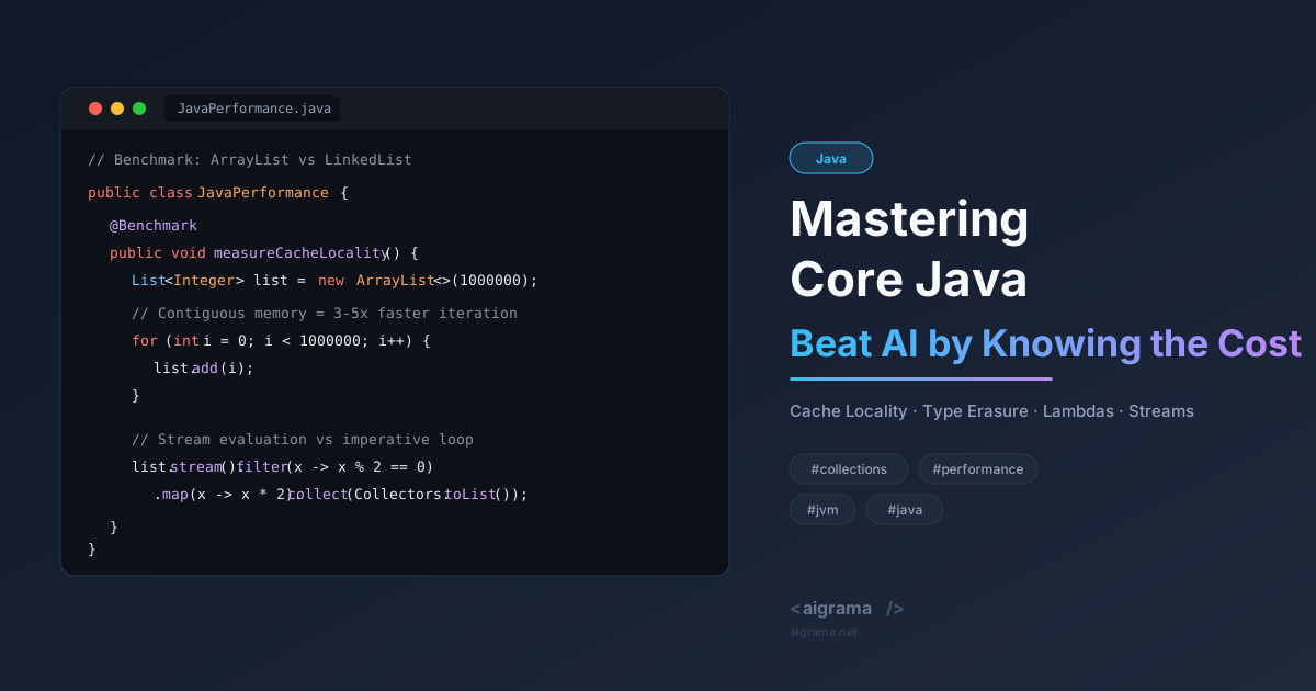
Mastering Core Java & Modern Features: Beat AI by Knowing the Cost
Understand the internal mechanics, memory footprints, and CPU cache costs of Collections, Generics, Lambdas, and Streams to write high-performance Java code that outpaces AI assistants.
Moving from simply using modern Java features to understanding their cost and internal mechanics is where you consistently outpace AI assistants. While AI will happily generate code that works functionally, high-performance Java engineering demands knowing what happens under the hood—from CPU cache lines to bytecode instructions.
Here is a deep dive into the four foundational pillars of Core Java & Modern Features, complete with internal mechanics, memory profiles, hands-on benchmarks, and prompt engineering strategies.
Chapter 1Deep Dive: Core Java & Modern Features
Part A: Collections — Knowing the Cost of Data Structures
AI will happily suggest List<Item> items = new LinkedList<>();. Your job is to know why that is almost always the wrong choice in modern Java.
What to Master
- ArrayList vs. LinkedList Internals:
ArrayListis backed by a contiguousObject[]array.LinkedListis a doubly-linked chain ofNodeobjects, each holding references to the item, previous node, and next node. - CPU Cache Locality: This is the secret performance differentiator. Because
ArrayListstores elements contiguously in memory, the CPU can preload a cache line (typically 64 bytes) with multiple element references, resulting in extremely high L1/L2/L3 cache hit rates.LinkedListnodes are scattered across the heap, so each pointer traversal step is likely a cache miss. In practice, iterating aLinkedListcan be 3–5x slower than anArrayListdue to cache misses alone. - Memory Overhead: Every
LinkedListnode carries two additional pointers (forward and backward) plus an object header (12-16 bytes). Storing N integers in aLinkedListconsumes roughly 3x more memory than anArrayListholding the same data. - ArrayList Resizing: The default initial capacity is 10. When full, it grows by a factor of 1.5x (
newCapacity = oldCapacity + (oldCapacity >> 1)). This growth triggers an array copy (System.arraycopy), which is an $O(n)$ operation, but the amortized cost of adding $n$ elements remains $O(1)$.
Hands-On Exercise
Write a JMH (Java Microbenchmark Harness) benchmark that inserts 1,000,000 integers into both an ArrayList and a LinkedList, then iterates over them and calculates the sum. Measure the time and memory footprint (using Runtime.getRuntime().totalMemory() - Runtime.getRuntime().freeMemory() deltas). The results will be stark.
AI Prompting Strategy
Instead of asking “When should I use ArrayList vs LinkedList?”, ask the AI:
“Generate a JMH benchmark to compare ArrayList and LinkedList for sequential iteration on a dataset of 1 million integers. Include memory allocation tracking.”
Then, analyze the results yourself and ask the AI to explain the discrepancy between theoretical Big-O complexity and observed execution performance.
Verification Check
Can you explain, without looking anything up, why iterating a
LinkedListis slower than anArrayListeven though both are $O(n)$?Answer: CPU cache locality. Contiguous memory allocation in
ArrayListallows CPU hardware prefetchers to load entire cache lines at once, whileLinkedListpointer chasing results in frequent L3 cache misses.
Part B: Generics — Understanding Type Erasure and Its Consequences
Generics in Java are a compile-time illusion. The JVM has no native knowledge of generic types. This design choice creates specific, real-world limitations you must be able to recognize and navigate.
What to Master
- Type Erasure: The compiler replaces all type parameters with their first bound (or
Objectif unbounded). At runtime,List<String>andList<Integer>are both just rawList. - No Runtime Type Information: You cannot execute
if (list instanceof List<String>). You cannot instantiatenew T(). You cannot overload methods that differ only by generic type parameter (e.g.,print(List<String>)andprint(List<Integer>)cause a compilation error due to identical signatures after erasure). - Bridge Methods: To preserve polymorphism after type erasure, the compiler generates synthetic “bridge methods.” For example, a class
StringBox extends Box<String>will have a compiler-generated synthetic methodset(Object)that casts toStringand delegates toset(String). These synthetic methods will appear in stack traces and reflection inspection. - Heap Pollution: Occurs when a variable of a parameterized type (e.g.,
List<String>) refers to an object that is not of that type (e.g.,List<Integer>). This typically occurs when mixing raw types with parameterized generics. The compiler emits an “unchecked warning.”
Hands-On Exercise
Write a generic method static <T> void addToList(List<T> list, T element) and invoke it with a raw List (e.g., List raw = new ArrayList(); addToList(raw, "hello");). Observe the compiler warning. Next, assign a raw list containing a String to a List<Integer>, retrieve the item, and inspect the resulting runtime ClassCastException.
AI Prompting Strategy
Ask the AI:
“Show me a code example that demonstrates heap pollution in Java generics and explain exactly which line triggers the unchecked warning and why the subsequent ClassCastException occurs.”
Verify the explanation against the Java Language Specification (JLS) or the official Oracle Generics tutorial.
Verification Check
Can you explain why
new T[]is illegal in Java?Answer: Because the JVM does not know what
Tis at runtime due to type erasure, and Java array creation requires explicit runtime type information to enforce array store safety.
Part C: Lambda Expressions — Understanding the invokedynamic Mechanism
AI can write a lambda expression in a fraction of a second. You need to understand that a lambda is not just “syntactic sugar” for an anonymous inner class. The underlying JVM bytecode mechanism is fundamentally different and carries its own performance profile.
What to Master
- Anonymous Inner Class vs. Lambda: An anonymous inner class generates a separate
.classfile at compile time (e.g.,Outer$1.class) and instantiates a new object on the heap upon execution. A lambda expression utilizes theinvokedynamic(indy) instruction. On first invocation,LambdaMetafactorydynamically generates a call site and links a class implementing the functional interface. Subsequent invocations reuse this call site without repeated class loading overhead. - Startup vs. Steady-State: The
invokedynamicapproach has a higher first-call overhead due to dynamic linkage and target resolution. However, for hot code paths, JVM JIT optimizations make lambdas perform equal to or better than anonymous inner classes, with a significantly smaller disk and memory footprint. - Capturing vs. Non-Capturing Lambdas: A non-capturing lambda (one that does not reference variables from its enclosing scope) can be cached as a singleton by the JVM, making allocations virtually free. A capturing lambda must allocate a new object instance on every invocation to hold captured variables.
Hands-On Exercise
Write a simple functional interface MyFunction with a method int apply(int a, int b). Create two implementations: one as an anonymous inner class, one as a lambda. Run your application with the JVM argument -Djava.lang.invoke.MethodHandle.TRACE_RESOLVE=true to observe the invokedynamic call site linkage in console output. Benchmark both approaches using JMH across cold-start and warm-up iterations.
AI Prompting Strategy
Ask the AI:
“Compare the performance characteristics of an anonymous inner class versus a lambda expression in Java, focusing on class loading, memory footprint, and the invokedynamic instruction. Show me a JMH benchmark that demonstrates the cold-start vs. steady-state difference.”
Verification Check
Can you explain why a lambda expression does not create a separate
.classfile at compile time, while an anonymous inner class does?Answer: Lambdas rely on
invokedynamicto defer class generation and instantiation to runtime viaLambdaMetafactory, whereas anonymous inner classes are compiled directly into standalone class files byjavac.
Part D: Stream API — Lazy Evaluation and the Hidden Cost of Convenience
AI tools love chaining .filter().map().sorted().collect(). You need to recognize when an elegant stream pipeline introduces unnecessary intermediate operations and memory pressure.
What to Master
- Lazy Evaluation: Intermediate operations (
filter,map) are lazy. They do not process elements until a terminal operation (collect,forEach,reduce) is invoked. This allows the Stream framework to fuse operations into a single iteration pass and support short-circuiting. - Stateless vs. Stateful Operations:
filterandmapare stateless; they process each element independently in a streaming fashion.sortedanddistinctare stateful; they must buffer all elements in memory before emitting a single element. Callingsorted()forces a full array copy of the stream’s contents, introducing significant allocation costs. - Stream vs. For-Loop Performance: For simple operations on smaller datasets (e.g., under 10,000 elements), a plain imperative
forloop is typically 3–4x faster than a Stream due to pipeline setup overhead, iterator allocation, and lambda invocation costs. For complex processing or massive datasets, Streams enhance maintainability. Parallel streams must be benchmarked carefully, as thread coordination overhead on the sharedForkJoinPool.commonPool()can easily make them slower than sequential streams. - Collector Memory Impact: The choice of
Collectordictates allocation efficiency.Collectors.toList()creates a standardArrayList.Collectors.toMap()requires duplicate key handling and instantiates aHashMap. TheCollectors.teeingcollector (introduced in Java 12) allows two downstream collectors to execute concurrently in a single pass.
Hands-On Exercise
Create a list of 1,000,000 Item objects (containing id, name, value). Benchmark three approaches using JMH:
- A traditional
forloop filtering, mapping, and collecting into anArrayList. - A sequential Stream pipeline:
list.stream().filter(...).map(...).collect(...). - A Stream pipeline with an added
.sorted()step before collection.
Observe how the sorted() variant causes a dramatic spike in execution time and garbage collection pressure.
AI Prompting Strategy
Ask the AI:
“Write a JMH benchmark that compares the performance and memory allocation of a for-loop versus a Java Stream pipeline for filtering and mapping a list of 1 million integers. Then, add a sorted() operation to the stream and explain why the performance degrades.”
Verification Check
Can you explain why
list.stream().map(String::toUpperCase).collect(Collectors.toList())might be slower than a simpleforloop for a list of 100 elements?Answer: For small collections, the overhead of stream pipeline instantiation, split-iterator creation, and generic lambda invocations outweighs the simple array indexing of an optimized
forloop.
Your Concrete “Beat the AI” Milestone for Chapter 1
After mastering these fundamentals, you will be equipped to review any AI-generated Java code and perform the following analysis:
- Identify the Data Structure: Explain why a chosen data structure (e.g.,
LinkedListvsArrayList) is optimal or sub-optimal based on cache line mechanics and memory footprint. - Spot Type Erasure Bugs: Inspect generic signatures and predict exact compiler warnings, bridge method generation, or runtime
ClassCastExceptionrisks. - Calculate Stream Costs: Evaluate stream pipelines to estimate total dataset passes and flag hidden memory allocations caused by stateful operations like
sorted(). - Benchmark and Prove: Write robust JMH benchmarks to validate your performance hypotheses using empirical JVM metrics rather than guesswork.
This level of deep mechanical understanding elevates you from someone who simply writes syntax into a software engineer who architects performance.
Chapter 2JVM Internals & Performance Tuning
Part A: JVM Memory Model — Heap vs. Stack
AI can explain the difference between Heap and Stack in one sentence. Your job is to understand the consequences of where objects live and how that affects application behavior.
What to Master:
- Stack Memory: Each thread has its own stack. It stores method call frames, local variables (primitives and object references), and partial results. Stack memory is fast because allocation and deallocation follow a strict LIFO (Last-In-First-Out) order—it’s just a pointer bump. The default stack size is typically 512KB–1MB per thread (
-Xss). StackOverflowError occurs when recursion goes too deep. - Heap Memory: Shared across all threads. It stores all objects and arrays created with
new. Heap-allocated data remains alive as long as it is reachable from a GC root (e.g., a local variable on a stack frame, a static field). The heap is divided into Young Generation (Eden + two Survivor spaces) and Old Generation (Tenured). New objects are allocated in Eden. Minor GC occurs when Eden fills up; surviving objects are promoted to Survivor spaces and eventually to the Old Generation. - Metaspace: Since Java 8, class metadata is stored in Metaspace, which uses native memory (not heap). It grows dynamically by default but can be bounded with
-XX:MaxMetaspaceSize. Unbounded Metaspace growth due to classloader leaks is a common production issue.
Hands-On Exercise:
Write a program that creates a large number of objects in a loop (e.g., new byte[1MB] in a loop). Run it with -Xmx64m -Xms64m and observe the OutOfMemoryError: Java heap space. Then, write a recursive method that never terminates and run it with -Xss256k to observe StackOverflowError. The difference in error messages and stack traces tells you which memory region is exhausted.
AI Prompting Strategy: Ask the AI: “Write a Java program that deliberately causes an OutOfMemoryError in the heap and a StackOverflowError in the stack. Show me the exact JVM flags to use and explain the stack trace differences.”
Verification Check:
Can you explain why local variables of primitive types are stored on the stack, but String objects are stored on the heap with only a reference on the stack? (Answer: Primitives are values stored directly in the stack frame; objects are always heap-allocated, and the stack holds only a reference to the heap location).
Part B: Garbage Collection Algorithms — G1 vs. ZGC
AI can list GC algorithms. You need to know which one to choose, when, and how to prove it with data.
What to Master:
- G1 (Garbage-First): The default server-side collector since JDK 9. It divides the heap into equal-sized regions and prioritizes collecting regions with the most garbage first. G1 targets a user-defined pause time (
-XX:MaxGCPauseMillis=200by default). It has a Stop-The-World (STW) Remark phase whose duration increases with heap size. G1 is a good balance of throughput and latency for heaps up to ~32GB. - ZGC (Z Garbage Collector): Introduced in JDK 11, designed for ultra-low latency (<10ms, often <1ms) and very large heaps (TB-scale). It performs almost all GC work concurrently with application threads, with only extremely short STW pauses. ZGC achieves this using colored pointers and load barriers. The trade-off: ZGC can have lower throughput than G1 in some workloads because it uses more CPU cycles for concurrent work. For example, a benchmark showed ZGC completing a task in 7.473s vs. G1’s 10.195s, but G1 often has higher raw throughput.
- Key Differentiator: For applications with strict tail-latency requirements (p99.9, p99.99), ZGC is dramatically better. For throughput-oriented batch processing, G1 or Parallel GC may be more efficient. For heaps under 4GB, the difference is often negligible.
Hands-On Exercise:
Write a simple Java application that allocates objects continuously and measures pause times. Run it with G1 (-XX:+UseG1GC) and ZGC (-XX:+UseZGC) separately. Enable GC logging with -Xlog:gc*:file=gc.log:time,uptime:filecount=5,filesize=10M. Compare the pause times in the logs. You will see G1 pauses spike during Remark, while ZGC pauses remain consistently tiny.
AI Prompting Strategy: Ask the AI: “Write a Java program that simulates a high-throughput workload with periodic large object allocations. Then, show me how to run it with both G1 and ZGC, and explain how to read the GC logs to compare pause times and throughput.”
Verification Check: Can you explain why ZGC has lower tail latency but potentially lower throughput than G1? (Answer: ZGC does more work concurrently, competing with application threads for CPU, which reduces throughput but eliminates long STW pauses).
Part C: Class Loading — The Hidden Source of Leaks
AI can explain the parent delegation model. You need to know how to detect and fix classloader leaks, which are a notoriously difficult class of memory problems.
What to Master:
- Class Loading Phases: Loading → Linking (Verification, Preparation, Resolution) → Initialization → Usage → Unloading. A class is loaded when it (or a subclass) is first accessed.
- Parent Delegation Model: The
ClassLoaderhierarchy is Bootstrap → Extension (Platform) → Application (System). When a class is requested, the parent loaders are asked first before the current loader attempts to load it. This ensures core Java classes are loaded by Bootstrap and prevents duplicates. - The Leak Scenario: A classloader leak occurs when a custom classloader (e.g., in a web container like Tomcat, or a plugin system) loads a class that creates a static reference or a ThreadLocal that outlives the classloader. The classloader cannot be garbage collected because the static reference (held by a GC root) points back to the class, which points to the classloader. Over time, repeated deployments (e.g., hot deployments) accumulate these leaked classloaders, leading to
OutOfMemoryError: Metaspace. - Detection:
jmap -clstats <pid>lists classloader statistics. If the count of classloaders keeps growing after redeployments, you have a leak.
Hands-On Exercise:
Write a custom ClassLoader that loads a simple class. Have the loaded class create a static final ThreadLocal or a static Map that holds a reference to an object. Then, discard all strong references to the classloader and call System.gc(). Use jmap -clstats to see if the classloader is still alive. If it is, you’ve reproduced a classloader leak.
AI Prompting Strategy: Ask the AI: “Show me a minimal Java example that demonstrates a classloader leak using a custom ClassLoader and a static field. Then, show me how to use jmap -clstats to detect that the classloader cannot be garbage collected.”
Verification Check: Can you explain why a static field in a class loaded by a custom classloader can prevent the classloader itself from being GC’d, even if all other references to the class are gone?
Part D: Diagnostic Tools — jstack, jmap, and Profilers
AI can tell you the syntax of jstack and jmap. You need to be able to interpret the output and draw conclusions about application health.
What to Master:
- jstack: Generates a thread dump. Use it to diagnose deadlocks, thread leaks, and high CPU usage. The output shows each thread’s state (
RUNNABLE,BLOCKED,WAITING), its stack trace, and any locks it holds or is waiting for. A thread dump is a snapshot; you often need multiple dumps seconds apart to identify a thread that is stuck in the same state. - jmap: Generates a heap dump (HPROF format) for offline analysis with tools like Eclipse MAT or VisualVM. Use
jmap -dump:format=b,file=heap.hprof <pid>for a full heap dump, orjmap -dump:live,format=b,file=heap.hprof <pid>to trigger a full GC first and dump only live objects. Note:jcmdis now recommended overjmapfor heap dumps because it is more reliable and does not require the JVM to be paused in the same way. - jcmd: A multi-purpose diagnostic tool. Useful commands:
jcmd <pid> GC.heap_info,jcmd <pid> GC.class_histogram,jcmd <pid> Thread.print,jcmd <pid> JFR.startfor Java Flight Recorder. - Profilers: Tools like Java Flight Recorder (JFR) (built into the JVM, low overhead) and Async Profiler (low-overhead CPU and allocation profiling) are essential for production diagnosis. JFR can record GC events, thread states, allocation samples, and more with less than 1% overhead.
Hands-On Exercise:
Start a Java application with -XX:+HeapDumpOnOutOfMemoryError -XX:HeapDumpPath=/tmp/heap.hprof. Trigger an OOM by allocating objects in a loop. After the OOM, open the generated heap.hprof in Eclipse MAT. Use the Dominator Tree to find the object retaining the most memory, and the Leak Suspects Report to identify the likely leak. Then, use jstack <pid> on a running application to find a deadlock: create two threads that each acquire two locks in opposite order.
AI Prompting Strategy: Ask the AI: “Walk me through the process of analyzing a heap dump from an OutOfMemoryError using Eclipse MAT. What is the difference between the Dominator Tree and the Histogram view? How do I use ‘Path to GC Roots’ to find the leak?”
Verification Check:
Can you explain the difference between jmap -dump:format=b,file=heap.hprof and jmap -dump:live,format=b,file=heap.hprof? (Answer: The live option triggers a full GC first and dumps only objects that are still reachable, which can make the dump smaller and more focused on actual leaks, but it pauses the JVM).
Your Concrete “Beat the AI” Milestone for Chapter 2
After working through this plan, you should be able to take a production OutOfMemoryError and do the following:
- Identify the Exhausted Region: Read the error message and determine whether it is Heap OOM (
Java heap space), Metaspace OOM (Metaspace), or Native OOM (unable to create new native thread). - Read a Heap Dump: Open an
.hproffile in Eclipse MAT, identify the dominator tree’s top object, and trace the GC root path to find the unintended retention. - Analyze a Thread Dump: Use
jstackto find a deadlock (threads inBLOCKEDstate waiting for locks held by each other) or a thread leak (hundreds of threads in the same state). - Tune GC Parameters: Given a workload profile, decide between G1 and ZGC, and set appropriate
-Xmx,-XX:MaxGCPauseMillis, and GC logging flags. - Explain It: Write a post-mortem report that explains the root cause, the fix, and the preventive measures (e.g., adding
-XX:+HeapDumpOnOutOfMemoryErrorto all production JVMs).
This level of understanding transforms you from someone who writes Java code into someone who keeps Java applications alive in production. That is the skill that remains indispensable in an AI-assisted world.
Suggested Practice Project
Use the diagnostic-lab project on GitHub as a sandbox for these exercises. It includes pre-built scenarios for memory leaks, deadlocks, and GC pressure. Run each scenario, capture the relevant dumps, and analyze them with the tools described above. This gives you reproducible, hands-on experience with the exact failure modes you will encounter in production.
Chapter 3Advanced Concurrency & Multithreading
Part A: Java Memory Model (JMM) — Visibility, Ordering, and Happens-Before
AI can write a volatile variable. You need to understand why it works and when it is insufficient. The JMM is the foundation of all concurrency reasoning.
What to Master:
-
The Three Pillars of Concurrency:
- Atomicity: An operation completes entirely or not at all.
count++is NOT atomic (it’s read-modify-write). - Visibility: Changes made by one thread are visible to another. Without synchronization, the JVM may cache variables in registers or CPU caches.
- Ordering: The compiler and CPU may reorder instructions for performance. The JMM defines when reordering is legal.
- Atomicity: An operation completes entirely or not at all.
-
Happens-Before Relationship: This is the core of the JMM. If action A happens-before action B, then A’s results are visible to B and A is ordered before B. Key rules:
- Program Order: Within a single thread, each action happens-before the next.
- Monitor Lock: An unlock on a monitor happens-before a subsequent lock on the same monitor.
- Volatile Variable: A write to a volatile field happens-before a subsequent read of that field.
- Thread Start:
Thread.start()happens-before any action in the started thread. - Thread Join: All actions in a thread happen-before another thread successfully returns from
join(). - Transitivity: If A → B and B → C, then A → C.
Visualization: Happens-Before in a Producer-Consumer Scenario
Thread A (Producer)                    Thread B (Consumer)
─────────────────                      ─────────────────
data = 42;          ──┐
                       │ (Program Order)
ready = true;       ──┘
                       │
                       │ (Volatile Write → Volatile Read)
                       ▼
                                    if (ready) {        ◄── Volatile Read
                                        print(data);    ◄── Guaranteed to see 42
                                    }

Without volatile on `ready`:
- Thread B might see `ready = true` but `data = 0` (reordered or cached).
- The write to `data` might not be flushed to main memory.
The Broken Double-Checked Locking Example (Pre-Java 5):
public class Singleton {
    private static Singleton instance;  // BROKEN without volatile

    public static Singleton getInstance() {
        if (instance == null) {                    // First check (no lock)
            synchronized (Singleton.class) {
                if (instance == null) {            // Second check (with lock)
                    instance = new Singleton();    // PROBLEM: This is not atomic
                }
            }
        }
        return instance;
    }
}
Why it’s broken: instance = new Singleton() involves three steps: (1) allocate memory, (2) initialize the object, (3) assign the reference. The JMM allows reordering of steps 2 and 3. So a thread could see a non-null instance that points to a partially constructed object. The fix is private static volatile Singleton instance;.
Hands-On Exercise:
Write a program with a shared boolean running = true (non-volatile) and a thread that loops while (running) {}. From the main thread, set running = false after 1 second. Run it on a multi-core machine. The loop may never terminate because the reader thread caches running in a register. Then, add volatile and observe it terminates reliably.
AI Prompting Strategy: Ask the AI: “Show me a Java program that demonstrates a visibility problem without volatile. Then, explain exactly which JMM rule is violated and how volatile fixes it. Include a timing diagram of the two threads.”
Verification Check:
Can you explain why volatile guarantees visibility but NOT atomicity for count++? (Answer: count++ is three operations—read, increment, write. Volatile ensures each read sees the latest value, but two threads can interleave their read-increment-write sequences, causing lost updates).
Part B: ExecutorService & Thread Pools — Sizing, Queues, and Rejection Policies
AI can create Executors.newFixedThreadPool(10). You need to know why that is often the wrong choice and how to size pools correctly.
What to Master:
-
Thread Pool Sizing Formula (Brian Goetz’s formula):
N_threads = N_cpu * U_cpu * (1 + W/C)Where
N_cpu= number of cores,U_cpu= target CPU utilization (0-1),W/C= ratio of wait time to compute time.- CPU-bound tasks (e.g., encryption):
N_threads = N_cpu + 1 - I/O-bound tasks (e.g., HTTP calls):
N_threads = N_cpu * (1 + wait_time/compute_time). For a task that waits 90ms and computes 10ms:N_threads = N_cpu * 10.
- CPU-bound tasks (e.g., encryption):
-
ThreadPoolExecutor Internals: When a task is submitted:
- If
corePoolSizethreads are not yet created, create a new thread. - If
corePoolSizethreads are busy, queue the task. - If the queue is full and
maxPoolSizeis not reached, create a new thread. - If
maxPoolSizeis reached and queue is full, invoke the Rejection Policy.
- If
-
Rejection Policies:
AbortPolicy(default): ThrowsRejectedExecutionException.CallerRunsPolicy: The submitting thread runs the task. Provides backpressure.DiscardPolicy: Silently drops the task. Dangerous.DiscardOldestPolicy: Drops the oldest queued task and retries.
-
Queue Choice Matters:
LinkedBlockingQueue(unbounded):maxPoolSizeis ignored because the queue never fills. Tasks queue indefinitely, leading to OOM.ArrayBlockingQueue(bounded): AllowsmaxPoolSizeto be effective. Provides backpressure.SynchronousQueue(zero capacity): Each task requires an available thread or a new one is created. Good forCachedThreadPool.
Visualization: ThreadPoolExecutor Task Flow
Task Submitted
      │
      ▼
┌─────────────────┐     Yes     ┌──────────────────┐
│ corePoolSize     │────────────►│ Create new thread│
│ threads busy?    │             └──────────────────┘
└────────┬────────┘
         │ No
         ▼
┌─────────────────┐     Yes     ┌──────────────────┐
│ Queue full?      │────────────►│ maxPoolSize      │
│                  │             │ reached?         │
└────────┬────────┘             └────────┬─────────┘
         │ No                            │ Yes
         ▼                               ▼
┌─────────────────┐             ┌──────────────────┐
│ Enqueue task     │             │ Rejection Policy │
└─────────────────┘             └──────────────────┘
Hands-On Exercise:
Create a ThreadPoolExecutor with corePoolSize=2, maxPoolSize=4, ArrayBlockingQueue(2), and CallerRunsPolicy. Submit 10 tasks that sleep for 1 second. Observe the behavior: tasks are processed by 2 core threads, then queued (2 tasks), then 2 more threads created (maxPoolSize=4), then the submitting thread runs the remaining tasks (backpressure). Log the thread name for each task to visualize the flow.
AI Prompting Strategy: Ask the AI: “Write a Java program using ThreadPoolExecutor with corePoolSize=2, maxPoolSize=4, ArrayBlockingQueue(2), and CallerRunsPolicy. Submit 10 tasks that log the thread name and sleep. Explain the exact sequence of thread creation, queuing, and rejection handling.”
Verification Check:
Can you explain why Executors.newFixedThreadPool(10) uses an unbounded LinkedBlockingQueue and why this can cause an OutOfMemoryError under load? (Answer: The unbounded queue never fills, so maxPoolSize is ignored and tasks accumulate until heap exhaustion).
Part C: Locks & Atomic Classes — CAS, Lock-Free Algorithms, and Contention
AI can write synchronized or ReentrantLock. You need to understand the trade-offs and when to use lock-free alternatives.
What to Master:
- synchronized vs. ReentrantLock:
| Feature | synchronized | ReentrantLock |
|---|---|---|
| Lock acquisition | Implicit | Explicit lock() / unlock() |
| Try-lock | No | tryLock(timeout) |
| Interruptible | No | lockInterruptibly() |
| Fairness | No | Optional fair=true |
| Condition variables | Single wait/notify | Multiple Condition objects |
| Performance (low contention) | Better (JVM optimizations) | Slightly worse |
| Performance (high contention) | Worse | Better (more control) |
-
Atomic Classes & CAS:
AtomicInteger,AtomicLong,AtomicReferenceuse Compare-And-Swap (CAS), a CPU instruction (e.g.,LOCK CMPXCHGon x86). CAS is lock-free but can suffer from the ABA problem and high contention spinning. -
The ABA Problem:
Thread 1: reads value A, prepares to CAS(A → C)
Thread 2: changes A → B, then B → A
Thread 1: CAS succeeds (sees A), but the state has changed underneath
Fix: Use
AtomicStampedReference(adds a version number). -
LongAdder vs. AtomicLong: Under high contention,
AtomicLongspins on CAS failures.LongAddermaintains multiple cells and sums them on read, drastically reducing contention. UseLongAdderfor high-throughput counters (e.g., metrics).
Visualization: CAS Retry Loop
Thread 1           Shared: AtomicInteger(5)        Thread 2
────────           ──────────────────────          ────────
read → 5                                           read → 5
CAS(5, 6) ──────►  value = 6  ✓
                                                   CAS(5, 6) ──► FAIL(value is 6)
                                                   re-read → 6
                                                   CAS(6, 7) ──► value = 7 ✓
Hands-On Exercise:
Write a benchmark comparing AtomicLong and LongAdder with 16 threads each incrementing 10 million times. Use JMH. LongAdder will be significantly faster under high contention because it avoids CAS retry storms.
AI Prompting Strategy: Ask the AI: “Write a JMH benchmark comparing AtomicLong and LongAdder with 16 threads incrementing 10 million times. Explain why LongAdder scales better under contention and show the internal cell-striping mechanism.”
Verification Check:
Can you explain why AtomicLong.incrementAndGet() can be slower than LongAdder.increment() under high contention? (Answer: AtomicLong uses a single CAS target, so all threads spin on the same memory location. LongAdder distributes updates across multiple cells, reducing contention).
Part D: CompletableFuture & Async Composition — Beyond Future.get()
AI can write CompletableFuture.supplyAsync(). You need to understand execution flow, error handling, and thread pool selection.
What to Master:
-
The Problem with
Future:Future.get()blocks. You cannot compose multiple futures without blocking.CompletableFuturesolves this with a monadic API (similar toOptionalorStream). -
Key Methods:
thenApply(Function): Transform result (sync).thenApplyAsync(Function): Transform result (async, uses ForkJoinPool or custom executor).thenCompose(Function): Chain anotherCompletableFuture(flatMap).thenCombine(other, BiFunction): Combine two independent futures.exceptionally(Function): Handle errors.handle(BiFunction): Handle both success and failure.allOf(futures): Wait for all to complete.anyOf(futures): Wait for the first to complete.
-
The Default Executor Trap:
thenApplyAsync()without an executor usesForkJoinPool.commonPool(), which hasN_cpu - 1threads. If you block on I/O inside acommonPooltask, you starve the pool. Always provide a custom executor for I/O-bound work.
Visualization: CompletableFuture Chaining
CompletableFuture.supplyAsync(() -> fetchUser(id), ioExecutor)   // Thread A
    .thenApplyAsync(user -> enrichUser(user), cpuExecutor)        // Thread B
    .thenComposeAsync(user -> fetchOrders(user), ioExecutor)      // Thread C
    .thenCombineAsync(
        CompletableFuture.supplyAsync(() -> fetchRecommendations(), ioExecutor),
        (orders, recs) -> new Dashboard(orders, recs)             // Thread D
    )
    .exceptionally(ex -> Dashboard.empty())                       // Error path
    .thenAccept(dashboard -> render(dashboard));                   // Final consumer
Hands-On Exercise:
Write a program that fetches data from three simulated APIs (each sleeps 1 second) using CompletableFuture. First, run them sequentially (3 seconds total). Then, run them in parallel with allOf (1 second total). Then, add error handling with exceptionally and observe the fallback path.
AI Prompting Strategy: Ask the AI: “Write a Java program that calls three simulated APIs in parallel using CompletableFuture.allOf(). Include error handling with exceptionally() and a custom executor for I/O tasks. Explain why using ForkJoinPool.commonPool() for blocking I/O is dangerous.”
Verification Check:
Can you explain the difference between thenApply and thenApplyAsync? (Answer: thenApply runs the function on the thread that completed the previous stage; thenApplyAsync submits the function to an executor).
Part E: Synchronization Strategies — Trade-offs and Deadlock Avoidance
AI can write a synchronized block. You need to choose the right strategy for the workload and avoid deadlocks.
What to Master:
- Lock Ordering: Always acquire locks in a consistent global order. Deadlock occurs when Thread 1 holds Lock A and waits for Lock B, while Thread 2 holds Lock B and waits for Lock A.
Visualization: Deadlock Cycle
Thread 1 ─── holds ───► Lock A
    │                      │
    │                      │ waits for
    ▼                      ▼
Lock B ◄─── waits ─── Thread 2
    │                      │
    │ holds                │
    ▼                      ▼
Thread 2 ─── waits ─── Lock A-
Lock Striping: Instead of one lock for a large data structure, use multiple locks for different segments.
ConcurrentHashMapuses this approach (though it now uses CAS + synchronized on nodes). -
ReadWriteLock: Allows multiple readers OR one writer. Good for read-heavy workloads. But beware:
ReentrantReadWriteLockcan suffer from writer starvation if readers are frequent.StampedLockoffers optimistic reads for even better performance. -
Thread Confinement: Avoid sharing state entirely. Use
ThreadLocalfor per-thread state (e.g.,SimpleDateFormatis not thread-safe; wrap it inThreadLocal). -
Immutability: The ultimate synchronization strategy. Immutable objects (e.g.,
String,Integer, records) are inherently thread-safe. Prefer immutability where possible.
Hands-On Exercise:
Write a program that creates a deadlock: two threads, two locks, acquired in opposite order. Use jstack <pid> to identify the deadlock. The thread dump will show Found one Java-level deadlock with the exact locks involved. Then, fix it by enforcing a global lock order.
AI Prompting Strategy: Ask the AI: “Write a Java program that creates a deadlock between two threads. Then, show me how to use jstack to identify the deadlock and explain the lock ordering fix.”
Verification Check:
Can you explain why ConcurrentHashMap does not use a single lock for the entire map? (Answer: It uses lock striping—different locks for different buckets—to allow concurrent writes to different segments).
Part F: Debugging Concurrency Issues — jcstress, Thread Dumps, and Stress Testing
AI cannot debug a race condition it cannot see. You need tools and techniques to reproduce and diagnose concurrency bugs.
What to Master:
-
jcstress (Java Concurrency Stress): A tool from OpenJDK for testing concurrency correctness. It runs millions of iterations with different thread interleavings to detect race conditions. Use it to validate lock-free algorithms.
-
Thread Dump Analysis for Concurrency:
jstack <pid>shows thread states.- Look for
BLOCKEDthreads (waiting for a monitor lock). - Look for
WAITINGthreads (waiting indefinitely, e.g.,Object.wait()). - Look for
TIMED_WAITINGthreads (e.g.,Thread.sleep()). - Multiple dumps seconds apart reveal threads stuck in the same state.
-
Java Flight Recorder (JFR): Records thread contention events (
jdk.JavaMonitorEnter,jdk.ThreadPark) with low overhead. Analyze with JDK Mission Control to find hot locks.
Hands-On Exercise:
Write a lock-free stack using AtomicReference and CAS. Run it through jcstress with a test that pushes and pops concurrently. jcstress will report any forbidden outcomes (e.g., losing elements). Then, introduce a bug (e.g., forget to use CAS correctly) and observe jcstress catch it.
AI Prompting Strategy: Ask the AI: “Write a lock-free stack in Java using AtomicReference and CAS. Then, write a jcstress test that pushes and pops concurrently and asserts that no elements are lost. Explain how jcstress detects race conditions.”
Verification Check:
Can you explain what a BLOCKED thread state means in a thread dump and how it differs from WAITING? (Answer: BLOCKED means waiting to acquire a monitor lock; WAITING means waiting indefinitely for another thread to perform a specific action, e.g., Object.wait() or Thread.join()).
Your Concrete “Beat the AI” Milestone for Chapter 3
After working through this plan, you should be able to take any concurrent code snippet (AI-generated or otherwise) and do the following:
- Identify the Synchronization Strategy: Determine whether it uses locks, CAS, thread confinement, or immutability, and explain the trade-offs.
- Spot Visibility Bugs: Look at a shared variable and determine whether it needs
volatile,synchronized, or an atomic class. - Reason About Happens-Before: Trace through a multi-threaded scenario and prove whether one thread’s writes are visible to another.
- Detect Deadlocks: Read a thread dump and identify the exact locks and threads involved in a deadlock cycle.
- Choose the Right Tool: Given a workload profile (CPU-bound vs. I/O-bound, low vs. high contention), select the appropriate executor, lock, or atomic class.
- Write a jcstress Test: Validate a lock-free algorithm with jcstress and interpret the results.
This level of understanding transforms you from someone who writes multi-threaded code into someone who engineers correct, high-performance concurrent systems. That is the skill that remains indispensable in an AI-assisted world.
Suggested Practice Project
Build a high-throughput, in-memory rate limiter using:
ConcurrentHashMapfor per-client counters.LongAdderfor high-contention counters.CompletableFuturefor async cleanup of expired entries.StampedLockfor optimistic reads of configuration.
Then, write a JMH benchmark comparing your implementation against a synchronized-based naive implementation. Use jstack to observe thread states under load, and use JFR to identify lock contention hotspots. This project touches every part of Chapter 3 and gives you a portfolio-ready artifact that demonstrates deep concurrency expertise.
Chapter 4System Design & Architecture Patterns
Part A: SOLID Principles — The Foundation of Maintainable Code
AI can generate a class that “works.” You need to recognize when a design will collapse under future requirements. SOLID is not academic theory—it is a practical framework for predicting maintenance cost.
What to Master:
-
Single Responsibility Principle (SRP): A class should have only one reason to change. This is about actors, not methods. A class that handles both business logic and persistence has two reasons to change: a business rule change and a database schema change.
-
Open/Closed Principle (OCP): Software entities should be open for extension but closed for modification. You should be able to add new behavior without editing existing, tested code.
-
Liskov Substitution Principle (LSP): Subtypes must be substitutable for their base types without breaking the program. The classic violation:
Square extends Rectangle—setting width on a square changes height, breaking the rectangle contract. -
Interface Segregation Principle (ISP): Clients should not be forced to depend on methods they do not use. A “fat” interface with 20 methods forces implementers to stub out irrelevant ones.
-
Dependency Inversion Principle (DIP): High-level modules should not depend on low-level modules; both should depend on abstractions. This is why we inject
PaymentGateway(interface) rather thanStripePaymentGateway(concrete class).
Visualization: SRP Violation vs. Fix
BEFORE (SRP Violation):
┌─────────────────────────────────────┐
│         OrderService                │
│  ─────────────────────────────────  │
│  + calculateTotal()                 │
│  + applyDiscount()                  │
│  + saveToDatabase()                 │  ◄── Persistence concern
│  + sendConfirmationEmail()          │  ◄── Notification concern
│  + generatePdfInvoice()             │  ◄── Reporting concern
└─────────────────────────────────────┘
        ▲
        │ Changes for: business rules, DB schema, email templates, PDF format
        │ → 4 reasons to change → fragile, hard to test

AFTER (SRP Applied):
┌──────────────────┐    ┌──────────────────┐    ┌──────────────────┐
│  OrderCalculator │    │  OrderRepository │    │  OrderNotifier   │
│  + calculate()   │    │  + save()        │    │  + sendEmail()   │
│  + applyDiscount()│   │  + findById()    │    │  + sendSms()     │
└──────────────────┘    └──────────────────┘    └──────────────────┘
        │                       │                       │
        ▼                       ▼                       ▼
   Business rules          DB schema              Notification
   changes only            changes only           changes only
Hands-On Exercise: Take a “God class” from a personal project (or generate one with AI) and refactor it using SRP. Identify each distinct actor (business stakeholder) that would request a change. Split the class so each actor has exactly one class to request changes from. Write unit tests for each new class—you will find they are dramatically simpler.
AI Prompting Strategy: Ask the AI: “Here is a class that handles order processing, database persistence, and email notifications. Identify the SRP violations and refactor it into separate classes. For each new class, explain which actor would request changes to it.” Then, verify the refactoring by asking: “What happens if we need to add SMS notifications? How many classes change?”
Verification Check:
Can you explain why Square extends Rectangle violates LSP? (Answer: Code that expects a Rectangle to have independent width and height will break when given a Square, because setting width also changes height).
Part B: Design Patterns — Strategy, Factory, Observer
AI can generate a pattern implementation. You need to know which pattern solves which problem and when a pattern is overkill.
What to Master:
- Strategy Pattern: Encapsulates interchangeable algorithms. Use when you have multiple ways to do something and want to select at runtime.
Visualization: Strategy Pattern
                    ┌─────────────────────┐
                    │   <<interface>>     │
                    │  PricingStrategy    │
                    │  + calculate(Order) │
                    └──────────┬──────────┘
                               │
          ┌────────────────────┼────────────────────┐
          │                    │                    │
          ▼                    ▼                    ▼
┌──────────────────┐ ┌──────────────────┐ ┌──────────────────┐
│ RegularPricing   │ │ PremiumPricing   │ │ DiscountPricing  │
│ + calculate()    │ │ + calculate()    │ │ + calculate()    │
└──────────────────┘ └──────────────────┘ └──────────────────┘

Client:
┌─────────────────────────────────────────────────────────┐
│  CheckoutService                                        │
│  ─────────────────────────────────────────────────────  │
│  private PricingStrategy strategy;  ◄── Injected        │
│  + checkout(order) { strategy.calculate(order); }       │
└─────────────────────────────────────────────────────────┘-
Factory Pattern: Centralizes object creation. Use when creation logic is complex or when you want to decouple clients from concrete implementations.
-
Observer Pattern: Defines a one-to-many dependency. When one object changes state, all dependents are notified. This is the foundation of event-driven architecture.
Visualization: Observer Pattern
┌─────────────────┐         ┌─────────────────────┐
│  OrderService   │────────►│  <<interface>>      │
│  (Subject)      │         │  OrderObserver      │
│  ─────────────  │         │  + onOrderPlaced()  │
│  - observers[]  │         └──────────┬──────────┘
│  + placeOrder() │                    │
│  + notify()     │      ┌─────────────┼─────────────┐
└─────────────────┘      │             │             │
                         ▼             ▼             ▼
                  ┌───────────┐ ┌───────────┐ ┌───────────┐
                  │ EmailSvc  │ │ Inventory │ │ Analytics │
                  │           │ │ Svc       │ │ Svc       │
                  └───────────┘ └───────────┘ └───────────┘
Hands-On Exercise:
Build a notification system that supports Email, SMS, and Push notifications. First, implement it with if/else branches. Then, refactor using the Strategy pattern. Then, add a new notification type (Slack) and observe: with if/else, you modify existing code; with Strategy, you add a new class without touching existing code (OCP).
AI Prompting Strategy: Ask the AI: “Show me a notification system implemented with if/else branches. Refactor it using the Strategy pattern. Then, demonstrate how adding a new notification type requires zero changes to existing classes with Strategy, but requires modification with if/else.”
Verification Check:
Can you explain when the Factory pattern is overkill? (Answer: When object creation is simple—new ArrayList<>() does not need a factory. Factories add value when creation involves configuration, conditional logic, or lifecycle management).
Part C: Monolith vs. Microservices — The Critical Decision
AI can generate a Spring Boot microservice. It cannot tell you whether you should build one. This is the most consequential architectural decision you will make, and it is almost always wrong to start with microservices.
What to Master:
-
Monolith First: Start with a modular monolith. Decompose into microservices only when you have a proven scaling or team autonomy bottleneck. The “MonolithFirst” pattern (Martin Fowler) is the industry consensus.
-
The Microservices Tax:
- Network latency: Every service call is a network hop (1-10ms) vs. an in-process method call (nanoseconds).
- Distributed debugging: A single request spans multiple services. You need distributed tracing (OpenTelemetry).
- Data consistency: No more ACID transactions across services. You need SAGA, eventual consistency, and idempotency.
- Operational complexity: Each service needs its own deployment pipeline, monitoring, logging, and on-call rotation.
-
When Microservices Are Justified:
- Independent scaling needs (e.g., search service needs 10x the instances of the auth service).
- Independent deployment cadence (e.g., teams deploy multiple times per day without coordinating).
- Technology heterogeneity (e.g., ML service in Python, core in Java).
- Organizational scaling (Conway’s Law: system architecture mirrors communication structure).
Visualization: Monolith vs. Microservices Trade-offs
                    MONOLITH                    MICROSERVICES
                    ────────                    ─────────────
Deployment          Single artifact             N artifacts
Latency             In-process (ns)             Network (ms)
Transactions        ACID                        SAGA / Eventual consistency
Debugging           Single stack trace          Distributed tracing required
Scaling             Vertical + horizontal       Per-service horizontal
Team structure      One team                    Multiple autonomous teams
Complexity          Low (initially)             High (always)
Best for            Startups, MVPs, <10 devs    Large orgs, proven scale needs
Decision Framework Visualization
                    Do you have a proven scaling bottleneck?
                              │
              ┌───────────────┴───────────────┐
              │ NO                            │ YES
              ▼                               ▼
    ┌─────────────────┐             ┌─────────────────┐
    │ Modular Monolith│             │ Do you have     │
    │ (Start here)    │             │ independent     │
    └─────────────────┘             │ team autonomy   │
                                    │ needs?          │
                                    └────────┬────────┘
                              ┌──────────────┴──────────────┐
                              │ NO                          │ YES
                              ▼                             ▼
                    ┌─────────────────┐           ┌─────────────────┐
                    │ Scale the       │           │ Extract        │
                    │ monolith        │           │ microservices  │
                    │ (horizontal)    │           │ incrementally  │
                    └─────────────────┘           └─────────────────┘
Hands-On Exercise:
Design a simple e-commerce system (users, products, orders, payments). First, design it as a modular monolith with clear module boundaries (packages: user, product, order, payment). Then, identify which modules could become services and what the data consistency challenges would be. Write down the exact network calls that would replace in-process method calls. Count the number of additional failure modes.
AI Prompting Strategy: Ask the AI: “Design an e-commerce system as a modular monolith with clear module boundaries. Then, for each module, explain what would be required to extract it as a microservice, including data consistency challenges, network failure modes, and operational overhead.”
Verification Check: Can you explain why starting with microservices for a new product is usually a mistake? (Answer: You do not yet know the domain boundaries. Premature decomposition leads to distributed monoliths—the worst of both worlds).
Part D: CAP Theorem & Data Consistency
AI can define CAP theorem. You need to apply it to real decisions about database selection and consistency models.
What to Master:
- CAP Theorem: In a distributed system, you can guarantee at most two of: Consistency, Availability, and Partition Tolerance. Since network partitions are inevitable, the real choice is between CP (consistency + partition tolerance) and AP (availability + partition tolerance).
Visualization: CAP Theorem Triangle
                        Consistency
                           /\
                          /  \
                         /    \
                        /      \
                       /   CA   \
                      /  (single \
                     /   node)    \
                    /              \
                   /────────────────\
                  /                  \
                 /                    \
                /         CP           \
               /      (HBase,          \
              /       MongoDB,          \
             /        Redis)             \
            /                            \
           /──────────────────────────────\
          /                                \
         /              AP                  \
        /         (Cassandra,               \
       /          DynamoDB,                  \
      /           CouchDB)                    \
     /──────────────────────────────────────────\
Availability ────────────────────────── Partition Tolerance-
CP Systems: Sacrifice availability during a partition. Example: A banking system where a partition means some ATMs refuse to dispense cash rather than risk showing an incorrect balance.
-
AP Systems: Sacrifice consistency during a partition. Example: A social media feed where a partition means you might see a slightly stale post, but the app remains available.
-
PACELC Extension: Even without partitions, there is a trade-off between Latency and Consistency. A strongly consistent system has higher latency because it must coordinate across nodes.
Real-World Example:
- PostgreSQL: CP (single-node, strongly consistent, unavailable during partition).
- Cassandra: AP (eventually consistent, always available, tunable consistency per query).
- MongoDB: CP (default), but configurable.
- DynamoDB: AP (eventually consistent reads by default, strongly consistent reads optional with higher latency).
Hands-On Exercise: Design a system with two features: (1) a user’s account balance, and (2) a user’s “likes” count on a post. For each feature, decide whether you need CP or AP. Justify your choice. Then, select a database for each and explain the trade-offs.
AI Prompting Strategy: Ask the AI: “Compare PostgreSQL, Cassandra, and DynamoDB in terms of CAP theorem. For each, give a real-world use case where it is the right choice and explain what is sacrificed.”
Verification Check: Can you explain why a banking system typically chooses CP over AP? (Answer: Showing an incorrect balance or allowing a double-spend is worse than briefly refusing service. Correctness > availability for financial transactions).
Part E: API Gateway Patterns
AI can generate a Spring Cloud Gateway route. You need to understand why an API gateway exists and what problems it solves—and what problems it creates.
What to Master:
- Why an API Gateway: Without one, every client must know the network location of every service, handle authentication independently, and manage cross-cutting concerns (rate limiting, logging, CORS). The gateway centralizes these concerns.
Visualization: API Gateway Architecture
                    ┌─────────────────────────────────────────┐
                    │           API Gateway                    │
                    │  ┌─────────────────────────────────┐    │
   ┌─────────┐     │  │  Auth    │ Rate     │ Routing  │    │
   │ Mobile  │─────┼──┤  Filter  │ Limiter  │ Filter   │    │
   └─────────┘     │  └─────────────────────────────────┘    │
                    └──────┬──────────┬──────────┬───────────┘
   ┌─────────┐           │          │          │
   │  Web    │───────────┘          │          │
   └─────────┘                      │          │
                           ┌────────▼──┐  ┌────▼──────┐  ┌──▼────────┐
                           │ User Svc  │  │ Order Svc │  │ Product   │
                           │           │  │           │  │ Svc       │
└───────────┘ └───────────┘ └───────────┘-
Gateway Responsibilities:
- Routing:
/api/users/**→ User Service,/api/orders/**→ Order Service. - Authentication: Validate JWT before forwarding. Services trust the gateway.
- Rate Limiting: Prevent abuse (e.g., 100 requests/minute per API key).
- Circuit Breaking: If Order Service is down, return a fallback instead of cascading failure.
- Request/Response Transformation: Add headers, redact sensitive fields.
- Routing:
-
BFF (Backend for Frontend) Pattern: Instead of one gateway for all clients, create one per client type. Mobile BFF returns compact JSON; Web BFF returns richer data. This avoids the “one-size-fits-all” API that serves no one well.
-
Anti-Pattern: Gateway as a God Service: If the gateway contains business logic (e.g., order calculation), it becomes a bottleneck and a deployment coordination point. Keep it thin.
Hands-On Exercise: Set up a Spring Cloud Gateway with three routes to three simple services. Add a JWT authentication filter and a rate limiter (using Redis). Then, simulate a service failure and configure a circuit breaker with a fallback response. Observe how the gateway isolates the failure from the client.
AI Prompting Strategy: Ask the AI: “Set up a Spring Cloud Gateway with JWT authentication, Redis-based rate limiting, and a CircuitBreaker filter with fallback. Explain the request flow and what happens when a downstream service is slow or down.”
Verification Check: Can you explain why putting business logic in the API gateway is an anti-pattern? (Answer: It couples all services to the gateway’s deployment cycle and creates a single point of failure for business logic).
Part F: SAGA Pattern & Distributed Transactions
AI can describe the SAGA pattern. You need to design a SAGA for a real business workflow and handle its failure modes.
What to Master:
-
The Problem: In a microservices architecture, you cannot use a single ACID transaction across services. A business operation (e.g., “place order”) spans multiple services (Order, Payment, Inventory, Shipping). If one step fails, you must undo the previous steps.
-
SAGA Pattern: A sequence of local transactions. Each step publishes an event or invokes the next step. If a step fails, compensating transactions are executed to undo the previous steps.
Visualization: SAGA Choreography vs. Orchestration
CHOREOGRAPHY (Event-Driven):
┌─────────┐    OrderCreated    ┌─────────┐   PaymentProcessed   ┌─────────┐
│ Order   │───────────────────►│ Payment │─────────────────────►│Inventory│
│ Service │                    │ Service │                      │ Service │
└─────────┘                    └─────────┘                      └─────────┘
     ▲                              │                                │
     │                              │ PaymentFailed                  │
     │     OrderCancelled           ▼                                │
     └──────────────────────── (compensating)                        │
                                                                     │
                                              InventoryReserved      │
                                                                     ▼
                                                              ┌─────────┐
                                                              │Shipping │
                                                              │ Service │
                                                              └─────────┘

ORCHESTRATION (Central Coordinator):
                    ┌─────────────────────────────────┐
                    │       Order Saga Orchestrator    │
                    │  ─────────────────────────────  │
                    │  1. createOrder()               │
                    │  2. processPayment()            │
                    │  3. reserveInventory()          │
                    │  4. arrangeShipping()           │
                    │  On failure: compensate()       │
                    └──────┬──────┬──────┬──────┬─────┘
                           │      │      │      │
                    ┌──────▼──┐ ┌─▼────┐ ┌▼─────┐ ┌▼──────┐
                    │ Order   │ │Payment│ │Invent│ │Shipping│
                    │ Service │ │Service│ │Service│ │Service│
└─────────┘ └──────┘ └──────┘ └───────┘-
Choreography: Services react to events. Decentralized, but hard to understand the overall flow. Good for simple sagas (2-3 steps).
-
Orchestration: A central orchestrator tells services what to do. Easier to understand, but the orchestrator can become a bottleneck. Good for complex sagas.
-
Compensating Transactions: Each step must have a compensating action:
- Create Order → Cancel Order
- Process Payment → Refund Payment
- Reserve Inventory → Release Inventory
- Arrange Shipping → Cancel Shipping
-
Idempotency: Every step and compensation must be idempotent. If a “Process Payment” message is delivered twice, the customer must not be charged twice. Use idempotency keys.
-
Semantic Lock: While a SAGA is in progress, the data is in an intermediate state. Other operations must be aware (e.g., “Order is PENDING, not CONFIRMED”). Use a state machine.
Hands-On Exercise: Design a SAGA for a travel booking system: (1) Book flight, (2) Book hotel, (3) Book car rental. If step 3 fails, compensate steps 2 and 1. Write the state machine for the order, including all intermediate states and compensating transitions. Identify where idempotency is required.
AI Prompting Strategy: Ask the AI: “Design a SAGA orchestrator for a travel booking system with flight, hotel, and car rental. Show the state machine, compensating transactions, and idempotency requirements. What happens if the compensation for the hotel booking fails?”
Verification Check: Can you explain why compensating transactions must be idempotent? (Answer: Because in a distributed system, messages can be delivered more than once. A non-idempotent refund would refund the customer twice).
Your Concrete “Beat the AI” Milestone for Chapter 4
After working through this plan, you should be able to take a business requirement and do the following:
- Design a Modular Monolith: Define module boundaries based on business capabilities, with clear interfaces between modules.
- Justify Microservices (or Not): Given a scaling or organizational bottleneck, explain whether microservices are the right solution and what the migration path looks like.
- Apply SOLID: Refactor a “God class” into cohesive, testable components, and explain the actors driving each change.
- Select a Design Pattern: Given a problem (e.g., multiple payment providers, complex object creation, event notification), choose the appropriate pattern and justify it.
- Apply CAP Theorem: Given a feature (e.g., account balance vs. social feed), choose CP or AP and select a database that matches.
- Design a SAGA: For a multi-step business workflow, design the orchestration, compensating transactions, and idempotency strategy.
- Draw the Architecture: Communicate the design using C4 diagrams (Context, Container, Component, Code) or similar.
This level of understanding transforms you from someone who writes code into someone who designs systems. That is the skill that remains indispensable in an AI-assisted world.
Suggested Practice Project
Build a modular monolith for a simplified e-commerce system with these modules:
user: registration, authentication, profile.product: catalog, search, inventory.order: cart, checkout, order lifecycle.payment: payment processing, refunds.
Define clear interfaces between modules. Write integration tests that verify module boundaries. Then, extract the payment module into a separate service and implement a SAGA for the checkout flow using either choreography (Kafka) or orchestration (a saga orchestrator). Document the trade-offs you experienced during the extraction—this document is your portfolio artifact demonstrating architectural maturity.
Chapter 5Database & SQL Mastery (Beyond CRUD)
Part A: Indexing Strategies — B-Tree, Hash, Composite, and Covering
AI can write CREATE INDEX idx_name ON users(name). You need to know which index to create, why it works, and when it will be ignored.
What to Master:
-
B-Tree Index (Default): The workhorse of relational databases. It stores data in a balanced tree structure, enabling O(log n) lookups, range scans, and ordered traversal. B-Tree indexes support:
=,<,>,BETWEEN,IN,LIKE 'prefix%', andORDER BY. -
Hash Index: Uses a hash function to map keys to bucket locations. O(1) lookup for exact equality only. Does NOT support range queries, sorting, or prefix matching. Used in PostgreSQL for equality-heavy columns, and internally by databases for hash joins.
-
Composite Index (Multi-Column): An index on multiple columns. The leftmost prefix rule is critical: an index on
(last_name, first_name)can be used for queries onlast_namealone, orlast_name + first_name, but NOT forfirst_namealone. -
Covering Index: An index that contains all columns needed by a query, so the database can answer the query entirely from the index without touching the table (called an “index-only scan”). This is one of the most powerful optimization techniques.
Visualization: B-Tree Index Structure
                    ┌─────────────────────┐
                    │     [50, 100]       │  ◄── Root Node
                    └──────┬──────┬───────┘
                           │      │
              ┌────────────┘      └────────────┐
              ▼                                ▼
       ┌─────────────┐                  ┌─────────────┐
       │  [20, 35]   │                  │ [75, 90]    │  ◄── Internal Nodes
       └──┬───┬───┬──┘                  └──┬───┬───┬──┘
          │   │   │                        │   │   │
     ┌────▼┐ ┌▼───┐ ┌▼───┐          ┌────▼┐ ┌▼───┐ ┌▼───┐
     │10,15│ │25,30│ │40,45│         │60,70│ │80,85│ │95,99│ ◄── Leaf Nodes
     └─────┘ └─────┘ └─────┘         └─────┘ └─────┘ └─────┘
         │       │       │               │       │       │
         ▼       ▼       ▼               ▼       ▼       ▼
      [rows]  [rows]  [rows]          [rows]  [rows]  [rows]
Visualization: Composite Index Leftmost Prefix Rule
Index: idx_name (last_name, first_name)

Query                                          Uses Index?
──────────────────────────────────────────────────────────
WHERE last_name = 'Smith'                      ✅ YES
WHERE last_name = 'Smith' AND first_name = 'John'  ✅ YES
WHERE first_name = 'John'                      ❌ NO (skips leftmost column)
WHERE first_name = 'John' AND last_name = 'Smith'  ✅ YES (optimizer reorders)
ORDER BY last_name, first_name                 ✅ YES
ORDER BY first_name                            ❌ NO
Visualization: Covering Index vs. Table Lookup
QUERY: SELECT email FROM users WHERE last_name = 'Smith';

WITHOUT COVERING INDEX (idx_last_name):
┌──────────────┐     ┌──────────────┐     ┌──────────────┐
│ Index Seek   │────►│ Table Lookup │────►│ Return email │
│ (find Smith) │     │ (fetch row)  │     │              │
└──────────────┘     └──────────────┘     └──────────────┘
                     ▲
                     │ Random I/O — expensive!

WITH COVERING INDEX (idx_last_name_email ON users(last_name, email)):
┌──────────────────────────────────────────────┐
│ Index-Only Scan                              │
│ (email is already in the index — no table!)  │
└──────────────────────────────────────────────┘
                     ▲
                     │ Sequential I/O — fast!
Hands-On Exercise:
Create a users table with 1,000,000 rows (use generate_series in PostgreSQL). Create an index on last_name. Run EXPLAIN ANALYZE SELECT email FROM users WHERE last_name = 'Smith'. Note the “Heap Fetches” (table lookups). Then, create a covering index on (last_name, email) and re-run. Observe the plan change to “Index Only Scan” and the execution time drop dramatically.
AI Prompting Strategy: Ask the AI: “Create a PostgreSQL table with 1 million rows. Show me the EXPLAIN ANALYZE output for a query with and without a covering index. Explain the difference between ‘Index Scan’ and ‘Index Only Scan’ and why ‘Heap Fetches’ matter.”
Verification Check:
Can you explain why an index on (last_name, first_name) cannot be used for a query that filters only on first_name? (Answer: B-Tree indexes are ordered by the leftmost column first. Without a value for last_name, the index cannot be traversed efficiently).
Part B: Query Execution Plans — Reading EXPLAIN Like a Pro
AI can generate a query. You need to read the execution plan and identify the bottleneck. EXPLAIN is your window into the database’s mind.
What to Master:
-
EXPLAIN vs. EXPLAIN ANALYZE:
EXPLAINshows the estimated plan.EXPLAIN ANALYZEactually executes the query and shows actual timings and row counts. Always useANALYZEfor diagnosis. -
Scan Types (from best to worst):
- Index Only Scan: Reads only the index. Fastest.
- Index Scan: Reads the index, then fetches matching rows from the table.
- Bitmap Index Scan + Bitmap Heap Scan: Builds a bitmap of matching rows, then reads the table in physical order. Good for medium-selectivity queries.
- Sequential Scan (Seq Scan): Reads the entire table. Slow for large tables, but sometimes faster than an index scan if the query returns a large percentage of rows.
-
Join Types:
- Nested Loop: For each row in the outer table, scan the inner table. Good for small datasets with an index on the inner table’s join column.
- Hash Join: Builds a hash table from the smaller table, then probes it with the larger table. Good for large, unsorted datasets.
- Merge Join: Sorts both tables and merges them. Good when both inputs are already sorted (e.g., from indexes).
-
Key Metrics to Look For:
- Estimated vs. Actual Rows: A large discrepancy means stale statistics. Run
ANALYZE table_name. - Cost: An arbitrary unit. Compare relative costs between plans, not absolute values.
- Actual Time: Milliseconds spent in each node. The node with the highest actual time is your bottleneck.
- Rows Removed by Filter: How many rows were discarded. High numbers indicate a missing or ineffective index.
- Estimated vs. Actual Rows: A large discrepancy means stale statistics. Run
Visualization: Reading an EXPLAIN ANALYZE Plan
QUERY: SELECT * FROM orders WHERE customer_id = 123 AND status = 'PENDING';

┌─────────────────────────────────────────────────────────────────────────────┐
│  Seq Scan on orders  (cost=0.00..25000.00 rows=1 width=100)                │
│                     (actual time=0.015..450.123 rows=3 loops=1)             │
│    Filter: ((customer_id = 123) AND (status = 'PENDING'))                   │
│    Rows Removed by Filter: 999997                                           │
│                                                                             │
│  ◄── Sequential Scan: reads ALL 1M rows                                     │
│  ◄── Estimated rows: 1, Actual rows: 3 (statistics are stale!)             │
│  ◄── Rows Removed: 999,997 (the index is missing or not used)               │
│  ◄── Actual time: 450ms (this is the bottleneck)                            │
└─────────────────────────────────────────────────────────────────────────────┘

AFTER adding index idx_orders_customer_status ON orders(customer_id, status):

┌─────────────────────────────────────────────────────────────────────────────┐
│  Index Scan using idx_orders_customer_status on orders                      │
│    (cost=0.42..12.46 rows=3 width=100)                                      │
│    (actual time=0.025..0.030 rows=3 loops=1)                                │
│    Index Cond: ((customer_id = 123) AND (status = 'PENDING'))               │
│                                                                             │
│  ◄── Index Scan: jumps directly to matching rows                            │
│  ◄── Actual time: 0.030ms (15,000x faster!)                                 │
└─────────────────────────────────────────────────────────────────────────────┘
Hands-On Exercise:
Create an orders table with 1,000,000 rows. Run a query filtering on a non-indexed column and capture EXPLAIN ANALYZE. Note the “Seq Scan” and high “Rows Removed by Filter.” Add an appropriate index. Re-run EXPLAIN ANALYZE. Observe the plan change and the execution time drop. Then, deliberately make the query non-sargable (e.g., WHERE UPPER(status) = 'PENDING') and observe the index is ignored. Fix it by creating an expression index.
AI Prompting Strategy: Ask the AI: “Show me an EXPLAIN ANALYZE plan for a slow query. Identify the bottleneck, explain what ‘Rows Removed by Filter’ means, and show me how to fix it with an index. Then, show me a non-sargable query that ignores the index and how to fix it with an expression index.”
Verification Check:
Can you explain why WHERE YEAR(created_at) = 2024 cannot use an index on created_at? (Answer: The function YEAR() is applied to the column, making it non-sargable. The index stores the raw created_at value, not the year. Rewrite as WHERE created_at >= '2024-01-01' AND created_at < '2025-01-01').
Part C: Transaction Isolation Levels — Real-World Impact
AI can explain the four isolation levels. You need to understand the concrete anomalies they prevent and the performance cost of each.
What to Master:
-
The Four Isolation Levels (from weakest to strongest):
- Read Uncommitted: Can see uncommitted changes from other transactions (dirty reads). Rarely used.
- Read Committed: Only sees committed changes. Default in PostgreSQL, Oracle, SQL Server. Prevents dirty reads, but allows non-repeatable reads and phantom reads.
- Repeatable Read: Once you read a row, it cannot change for the duration of the transaction. Default in MySQL InnoDB. Prevents dirty reads and non-repeatable reads, but allows phantom reads (in theory; InnoDB prevents them with gap locks).
- Serializable: Transactions appear to execute sequentially. Prevents all anomalies. Highest cost due to locking or serialization conflicts.
-
The Three Anomalies:
- Dirty Read: Reading uncommitted data from another transaction.
- Non-Repeatable Read: Reading the same row twice and getting different values because another transaction committed a change in between.
- Phantom Read: Running the same query twice and getting different sets of rows because another transaction inserted or deleted rows in between.
Visualization: Isolation Levels vs. Anomalies
                    Dirty    Non-Repeatable    Phantom
                    Read     Read              Read
─────────────────────────────────────────────────────────
Read Uncommitted    ❌       ❌                ❌
Read Committed      ✅       ❌                ❌
Repeatable Read     ✅       ✅                ❌*
Serializable        ✅       ✅                ✅

✅ = Prevented    ❌ = Possible
* MySQL InnoDB prevents phantoms via gap locks
Visualization: Non-Repeatable Read in Action
Time    Transaction A (Read Committed)          Transaction B
────    ──────────────────────────────          ─────────────
T1      BEGIN;
T2      SELECT balance FROM accounts
        WHERE id = 1;
        ──► balance = 1000
T3                                              BEGIN;
T4                                              UPDATE accounts SET balance = 500
                                                WHERE id = 1;
T5                                              COMMIT;
T6      SELECT balance FROM accounts
        WHERE id = 1;
        ──► balance = 500  ◄── Different value! Non-repeatable read.
T7      COMMIT;
Hands-On Exercise:
Open two psql sessions. In Session A, set SET TRANSACTION ISOLATION LEVEL READ COMMITTED; and begin a transaction. Read a row. In Session B, update that row and commit. In Session A, read the row again—you will see the new value (non-repeatable read). Repeat with REPEATABLE READ—you will see the original value. Then, test phantom reads by inserting new rows that match a WHERE clause and re-running the query.
AI Prompting Strategy: Ask the AI: “Write a step-by-step SQL script using two sessions to demonstrate a non-repeatable read under READ COMMITTED and show how REPEATABLE READ prevents it. Then, demonstrate a phantom read and explain how SERIALIZABLE prevents it.”
Verification Check: Can you explain why PostgreSQL’s default is Read Committed while MySQL’s default is Repeatable Read? (Answer: Historical and philosophical differences. PostgreSQL prioritizes concurrency and uses MVCC with snapshots; MySQL InnoDB uses gap locks and next-key locks to prevent phantoms even at Repeatable Read).
Part D: Connection Pooling — The Hidden Bottleneck
AI can configure HikariCP with default settings. You need to understand pool sizing, connection lifecycle, and common failure modes.
What to Master:
-
Why Pooling: Creating a database connection is expensive (TCP handshake, authentication, session setup). A pool reuses connections, amortizing this cost. Typical connection creation: 20-50ms. Pool checkout: <1ms.
-
Pool Sizing Formula (HikariCP’s recommendation):
connections = ((core_count * 2) + effective_spindle_count)For a 4-core machine with SSD:
(4 * 2) + 1 = 9connections. Not 100. More connections do NOT mean more throughput—they mean more context switching and lock contention inside the database.
Visualization: Connection Pool Architecture
┌─────────────────────────────────────────────────────────────────────────────┐
│                           Application                                        │
│  ┌─────────┐  ┌─────────┐  ┌─────────┐  ┌─────────┐  ┌─────────┐           │
│  │Thread 1 │  │Thread 2 │  │Thread 3 │  │Thread 4 │  │Thread 5 │           │
│  └────┬────┘  └────┬────┘  └────┬────┘  └────┬────┘  └────┬────┘           │
│       │            │            │            │            │                 │
│       ▼            ▼            ▼            ▼            ▼                 │
│  ┌─────────────────────────────────────────────────────────────────────┐    │
│  │                    HikariCP Connection Pool                         │    │
│  │  ┌──────┐ ┌──────┐ ┌──────┐ ┌──────┐ ┌──────┐ ┌──────┐ ┌──────┐    │    │
│  │  │Conn 1│ │Conn 2│ │Conn 3│ │Conn 4│ │Conn 5│ │Conn 6│ │Conn 7│    │    │
│  │  └──┬───┘ └──┬───┘ └──┬───┘ └──┬───┘ └──┬───┘ └──┬───┘ └──┬───┘    │    │
│  └─────┼────────┼────────┼────────┼────────┼────────┼────────┼────────┘    │
│        │        │        │        │        │        │        │             │
└────────┼────────┼────────┼────────┼────────┼────────┼────────┼─────────────┘
         │        │        │        │        │        │        │
         ▼        ▼        ▼        ▼        ▼        ▼        ▼
┌─────────────────────────────────────────────────────────────────────────────┐
│                        PostgreSQL (max_connections = 100)                    │
│   Each connection = 1 process, ~10MB memory, context switch overhead        │
└─────────────────────────────────────────────────────────────────────────────┘- Key HikariCP Settings:
maximumPoolSize: Max connections. Start with the formula above, then tune.minimumIdle: Connections kept idle. Set equal tomaximumPoolSizefor fixed pools (avoids latency spikes).connectionTimeout: How long a thread waits for a connection. Default 30s. If you see timeouts, your pool is too small OR connections are held too long.maxLifetime: Max age of a connection. Should be less than the database’swait_timeout(e.g., 30 minutes for MySQL). Prevents “connection closed” errors.leakDetectionThreshold: Logs a warning if a connection is held longer than this. Set to 2x your longest expected query. Invaluable for finding connection leaks.
Visualization: Connection Leak
Time    Thread 1                          Connection Pool
────    ────────                          ───────────────
T1      getConnection() ──────────────────► Conn 1 (checked out)
T2      executeQuery()                      Conn 1 (in use)
T3      ... exception thrown ...            Conn 1 (still checked out!)
T4      (no finally block, no close())      Conn 1 (leaked)
T5      getConnection() ──────────────────► Conn 2 (checked out)
T6      ...                                 Conn 2 (leaked)
...
T100    getConnection() ──────────────────► TIMEOUT! Pool exhausted.
Hands-On Exercise:
Configure HikariCP with maximumPoolSize=5 and leakDetectionThreshold=2000. Write a method that gets a connection, executes a query, and deliberately forgets to close it (simulate an exception path without a finally block). Call this method 6 times. Observe the pool exhaustion and the leak detection warning in the logs. Then, fix it with try-with-resources and observe the pool recover.
AI Prompting Strategy: Ask the AI: “Configure HikariCP with a maximum pool size of 5 and leak detection threshold of 2 seconds. Write a Java method that demonstrates a connection leak by not closing the connection on an exception path. Show me the log output and explain how to fix it with try-with-resources.”
Verification Check:
Can you explain why setting maximumPoolSize=100 for a 4-core database server is counterproductive? (Answer: The database can only execute as many queries in parallel as it has cores. Extra connections queue inside the database, consuming memory and causing context switches, which reduces throughput).
Part E: Query Optimization Patterns — Beyond Indexes
AI can suggest “add an index.” You need to recognize when the query itself is the problem.
What to Master:
- N+1 Query Problem: Fetching a list of N items, then executing N additional queries for related data. The fix: use a JOIN or a batch fetch. This is the most common ORM performance killer.
Visualization: N+1 Problem
NAIVE (N+1 queries):
┌─────────────────────────────────────────────────────────────────┐
│  SELECT * FROM orders;                          ──► 100 orders │
│  SELECT * FROM customers WHERE id = 1;          ──► 1 query    │
│  SELECT * FROM customers WHERE id = 2;          ──► 1 query    │
│  ...                                                             │
│  SELECT * FROM customers WHERE id = 100;        ──► 1 query    │
│                                                                  │
│  Total: 101 queries, 101 round trips                            │
└─────────────────────────────────────────────────────────────────┘

OPTIMIZED (JOIN):
┌─────────────────────────────────────────────────────────────────┐
│  SELECT o.*, c.* FROM orders o                                  │
│  JOIN customers c ON o.customer_id = c.id;      ──► 1 query    │
│                                                                  │
│  Total: 1 query, 1 round trip                                   │
└─────────────────────────────────────────────────────────────────┘- Pagination Done Wrong:
OFFSET 1000000 LIMIT 10forces the database to scan and discard 1,000,000 rows. The fix: keyset pagination (also called cursor pagination) using aWHERE id > last_seen_idclause.
Visualization: OFFSET vs. Keyset Pagination
OFFSET PAGINATION (slow):
SELECT * FROM orders ORDER BY id LIMIT 10 OFFSET 1000000;
┌─────────────────────────────────────────────────────────────────┐
│  Scan 1,000,000 rows ──► Discard them ──► Return 10 rows        │
│  Time: 2.5 seconds                                               │
└─────────────────────────────────────────────────────────────────┘

KEYSET PAGINATION (fast):
SELECT * FROM orders WHERE id > 1000000 ORDER BY id LIMIT 10;
┌─────────────────────────────────────────────────────────────────┐
│  Index seek to id=1000000 ──► Return next 10 rows               │
│  Time: 0.5 milliseconds                                          │
└─────────────────────────────────────────────────────────────────┘-
SELECT * Anti-Pattern: Fetches all columns, including large BLOBs or TEXT fields you do not need. This increases I/O, network transfer, and memory. Always select only the columns you need.
-
Implicit Type Conversion:
WHERE user_id = '123'(string) whenuser_idis an integer forces a cast on every row, preventing index usage. Always match the column type.
Hands-On Exercise:
Create an orders table and a customers table with 100,000 rows each. Write a Java program using JDBC (or JPA) that fetches all orders and then fetches each customer individually (N+1). Measure the time. Then, rewrite it with a single JOIN query. Measure again. Then, test OFFSET 50000 LIMIT 10 vs. keyset pagination and compare execution times.
AI Prompting Strategy: Ask the AI: “Write a Java program that demonstrates the N+1 query problem with JPA. Then, show me how to fix it with a JOIN FETCH query. Benchmark both approaches and explain the performance difference.”
Verification Check:
Can you explain why OFFSET 1000000 LIMIT 10 is slow even with an index on the ORDER BY column? (Answer: The database must still traverse the index to skip 1,000,000 entries. Keyset pagination uses the index to seek directly to the starting point).
Your Concrete “Beat the AI” Milestone for Chapter 5
After working through this plan, you should be able to take a slow query and do the following:
- Read an Execution Plan: Identify Seq Scans, high “Rows Removed by Filter,” and estimated vs. actual row discrepancies.
- Design the Right Index: Choose between B-Tree, Hash, Composite, and Covering indexes based on the query pattern.
- Detect Non-Sargable Queries: Spot functions on columns, implicit type conversions, and leading wildcards that prevent index usage.
- Choose an Isolation Level: Given a business requirement (e.g., financial transaction vs. social feed), select the appropriate isolation level and explain the trade-offs.
- Size a Connection Pool: Apply the formula, configure HikariCP, and detect connection leaks.
- Fix N+1 Queries: Identify them in ORM logs and rewrite with JOINs or batch fetching.
- Implement Keyset Pagination: Replace OFFSET-based pagination for large datasets.
- Prove It with EXPLAIN ANALYZE: Before and after every optimization, capture the execution plan and the actual timing.
This level of understanding transforms you from someone who writes queries into someone who engineers data access. That is the skill that remains indispensable in an AI-assisted world.
Suggested Practice Project
Build a query optimization lab using PostgreSQL and a Java application:
- Schema: Create
users,orders,order_items, andproductstables with realistic data (1M+ rows). Usegenerate_seriesand random data generators. - Slow Queries: Write 5 deliberately slow queries:
- A query with no index.
- A query with a non-sargable predicate.
- A query with
SELECT *on a table with large TEXT columns. - An N+1 query via JPA.
- An OFFSET-based pagination query at a high offset.
- Optimize Each: For each query, capture
EXPLAIN ANALYZE, apply the fix (index, rewrite, JOIN, keyset pagination), and capture the new plan. Document the before/after timing. - Connection Pool: Configure HikariCP, demonstrate a connection leak, and fix it.
- Isolation Levels: Write a script that demonstrates a non-repeatable read and a phantom read, then show how higher isolation levels prevent them.
This project gives you a portfolio-ready artifact demonstrating deep database expertise—the kind that AI cannot generate because it requires iterating against a real database with real data distribution.
Chapter 6Distributed Systems & Event-Driven Architecture
Part A: Message Brokers — Kafka vs. RabbitMQ
AI can write a @KafkaListener or a @RabbitListener. You need to know which broker to choose, why, and how their internal architectures dictate their behavior under failure.
What to Master:
-
Kafka’s Architecture: A distributed, partitioned, replicated commit log. Messages are appended to partitions and retained for a configurable period (or forever). Consumers track their position via offsets. Key properties:
- Pull-based: Consumers pull at their own pace. Natural backpressure.
- Ordering: Guaranteed within a partition, not across partitions.
- Replay: Consumers can seek to any offset and reprocess. This is impossible in traditional queues.
- Throughput: Sequential disk I/O + zero-copy transfer = millions of messages/sec.
-
RabbitMQ’s Architecture: A traditional message broker with exchanges, queues, and bindings. Messages are pushed to consumers and removed once acknowledged. Key properties:
- Push-based: Broker pushes messages. Uses prefetch limits for backpressure.
- Flexible routing: Exchanges (direct, topic, fanout, headers) route messages to queues based on routing keys.
- Per-message acknowledgment: Fine-grained control over message lifecycle.
- Lower latency: For low-volume, low-latency workloads, RabbitMQ often wins.
Visualization: Kafka vs. RabbitMQ Architecture
KAFKA (Distributed Commit Log):
┌─────────────────────────────────────────────────────────────────────────────┐
│  Topic: orders (3 partitions, replication factor 2)                         │
│                                                                             │
│  Partition 0: [msg0][msg3][msg6][msg9]...  ──► Consumer Group A             │
│  Partition 1: [msg1][msg4][msg7][msg10]... ──► Consumer Group A             │
│  Partition 2: [msg2][msg5][msg8][msg11]... ──► Consumer Group A             │
│                                                                             │
│  Offset:        0    1    2    3    4    5                                  │
│  Retention:     7 days (configurable, replayable)                           │
│  Ordering:      Per-partition only                                          │
│  Replay:        Yes (seek to any offset)                                    │
└─────────────────────────────────────────────────────────────────────────────┘

RABBITMQ (Exchange → Queue → Consumer):
┌─────────────────────────────────────────────────────────────────────────────┐
│                                                                             │
│  Producer ──► Exchange ──┬──► Queue A ──► Consumer 1 (acknowledges)         │
│  (routing key)           │                                                  │
│                          ├──► Queue B ──► Consumer 2 (acknowledges)         │
│                          │                                                  │
│                          └──► Queue C ──► Consumer 3 (acknowledges)         │
│                                                                             │
│  Exchange Types: Direct, Topic, Fanout, Headers                             │
│  Ordering:       Per-queue                                                   │
│  Replay:         No (message removed after ack)                             │
│  Push-based:     Broker pushes, prefetch limits backpressure                │
└─────────────────────────────────────────────────────────────────────────────┘
Decision Matrix:
| Requirement | Kafka | RabbitMQ |
|---|---|---|
| High throughput (>100K msg/sec) | ✅ Best | ❌ Limited |
| Message replay / event sourcing | ✅ Native | ❌ Not supported |
| Complex routing (topic, headers) | ⚠️ Manual | ✅ Native |
| Low latency (<10ms) | ⚠️ Batching adds latency | ✅ Best |
| Per-message TTL / delayed messages | ❌ Not native | ✅ Native |
| Long-term retention | ✅ Days/weeks/forever | ❌ Until consumed |
| Ordered processing per key | ✅ Per-partition | ✅ Per-queue |
Hands-On Exercise: Set up a local Kafka (using Docker) and RabbitMQ. Write a producer that sends 100,000 messages to each. Write a consumer that reads and processes them. Measure throughput and latency. Then, kill the consumer mid-stream and restart it. Observe: Kafka resumes from the last committed offset (no message loss, possible reprocessing); RabbitMQ redelivers unacknowledged messages (possible duplicates, no loss if ack is used correctly).
AI Prompting Strategy: Ask the AI: “Write a Docker Compose file for Kafka and RabbitMQ. Then, write a Java producer and consumer for each. Benchmark throughput and latency, and explain what happens to in-flight messages when the consumer crashes and restarts.”
Verification Check: Can you explain why Kafka guarantees ordering only within a partition, not across partitions? (Answer: Partitions are independent logs. Messages in different partitions are written in parallel and have no global ordering. To guarantee ordering for a specific entity, you must route all its messages to the same partition, typically using the entity ID as the partition key).
Part B: Idempotency — The Cornerstone of Reliable Messaging
AI can write a consumer that processes a message. You need to ensure that processing it twice has the same effect as processing it once. In distributed systems, at-least-once delivery is the norm, so idempotency is not optional.
What to Master:
-
Why Duplicates Happen: A consumer processes a message, but the acknowledgment is lost due to a network partition. The broker redelivers the message. The consumer processes it again. Without idempotency, you get double-charging, double-emailing, or double-inventory-decrement.
-
Idempotency Key Pattern: Every message carries a unique
idempotency_key(e.g., a UUID generated by the producer). The consumer stores processed keys in a durable store (database table, Redis) and checks before processing.
Visualization: Idempotent Consumer Flow
Message arrives (idempotency_key = "abc-123")
              │
              ▼
┌─────────────────────────────┐
│  Check if key exists in     │
│  processed_messages table   │
└─────────────┬───────────────┘
              │
      ┌───────┴───────┐
      │               │
      ▼               ▼
   EXISTS          NOT EXISTS
      │               │
      ▼               ▼
┌───────────┐   ┌─────────────────────────────┐
│ Skip      │   │ BEGIN TRANSACTION            │
│ (already  │   │  - Process message           │
│ processed)│   │  - INSERT idempotency_key    │
└───────────┘   │  - Publish downstream event  │
                │ COMMIT                       │
└─────────────────────────────┘-
Database-Level Idempotency: Use a unique constraint on the idempotency key. If the insert fails with a duplicate key error, the message was already processed. This is atomic and race-condition-free.
-
Idempotent Operations: Some operations are naturally idempotent:
SET balance = 100(idempotent)UPDATE status = 'SHIPPED' WHERE id = 5(idempotent)INSERT INTO orders (id, ...) VALUES (5, ...)(idempotent ifidis unique)UPDATE balance = balance - 100(NOT idempotent—requires idempotency key)
Hands-On Exercise:
Write a Kafka consumer that processes “payment” events. Each event has a payment_id and an amount. The consumer deducts the amount from a customer’s balance. First, write it naively (UPDATE balance = balance - amount). Then, simulate a duplicate delivery by sending the same event twice. Observe the double deduction. Then, add an idempotency key table with a unique constraint and fix the issue.
AI Prompting Strategy: Ask the AI: “Write a Kafka consumer that processes payment events and deducts from a balance. Demonstrate the double-charging problem when the same event is delivered twice. Then, fix it using an idempotency key table with a unique constraint and a transaction.”
Verification Check:
Can you explain why UPDATE balance = balance - 100 is not idempotent, but UPDATE balance = 100 is? (Answer: The first decrements the balance each time it runs; the second sets it to a fixed value regardless of how many times it runs).
Part C: Dead Letter Queues & Error Handling — The Operational Reality
AI can write a try/catch block. You need to design a failure handling strategy that distinguishes between transient errors (retry), permanent errors (dead letter), and poison messages (quarantine + alert).
What to Master:
- Retry Strategy: Not all errors are equal.
- Transient errors (network timeout, database deadlock): Retry with exponential backoff. After N retries, move to DLQ.
- Permanent errors (invalid schema, business rule violation): Do NOT retry. Immediately move to DLQ and alert.
- Poison messages (cause consumer to crash repeatedly): Move to a quarantine topic after 1-2 attempts and alert a human.
Visualization: Retry + DLQ Flow
Message arrives
      │
      ▼
┌─────────────┐     Success     ┌──────────────┐
│  Process    │────────────────►│  Acknowledge │
│  Message    │                 └──────────────┘
└──────┬──────┘
       │ Failure
       ▼
┌─────────────────┐
│  Transient?     │
└────────┬────────┘
    ┌────┴────┐
    │         │
    ▼         ▼
  YES        NO
    │         │
    ▼         ▼
┌────────┐ ┌──────────────────────────────────────┐
│ Retry  │ │  Move to Dead Letter Queue (DLQ)     │
│ (backoff│ │  + Alert                              │
│  + max  │ │  + Preserve original message + error  │
│  retries│ │  + Metadata (timestamp, consumer,     │
│  )      │ │    stack trace, retry count)          │
└────┬───┘ └──────────────────────────────────────┘
     │
     │ Max retries exceeded
     ▼
┌──────────────────────────────────────┐
│  Move to DLQ                          │
│  + Alert                              │
└──────────────────────────────────────┘-
DLQ Message Contents: A DLQ message must contain:
- The original message payload (unmodified).
- The error message and stack trace.
- The consumer group and topic/partition/offset.
- The timestamp of the first failure and the number of attempts.
- A correlation ID for tracing.
-
DLQ Reprocessing: A DLQ is not a graveyard—it is a holding area. You need a strategy:
- Manual replay: An operator inspects the DLQ, fixes the root cause, and re-publishes the message.
- Automated replay: A scheduled job re-publishes DLQ messages after a delay (for transient errors).
- Discard: After a retention period, discard messages that are no longer relevant.
Hands-On Exercise:
Write a Kafka consumer with a retry mechanism: 3 retries with exponential backoff, then a DLQ. Inject a transient error (e.g., SocketTimeoutException) and observe the retries. Then, inject a permanent error (e.g., IllegalArgumentException) and observe immediate DLQ routing. Write a separate consumer for the DLQ topic that logs the message and error metadata.
AI Prompting Strategy: Ask the AI: “Write a Kafka consumer with a retry mechanism (3 retries, exponential backoff) and a dead letter queue. Differentiate between transient and permanent errors. Show the DLQ message structure and write a DLQ consumer that logs and alerts.”
Verification Check: Can you explain why a poison message should not be retried indefinitely? (Answer: It will crash the consumer repeatedly, blocking the entire partition and causing a backlog. Moving it to a DLQ unblocks the partition and allows a human to investigate).
Part D: Distributed Tracing — Seeing the Invisible
AI can add a log.info() statement. You need to trace a request across 10 services and identify the bottleneck. Distributed tracing is non-negotiable in a microservices architecture.
What to Master:
- The Three Pillars of Observability:
- Logs: Discrete events. Good for debugging specific issues. Bad for understanding request flow.
- Metrics: Aggregated numbers (CPU, latency, error rate). Good for alerting. Bad for root-cause analysis.
- Traces: The end-to-end journey of a request across services. Good for understanding latency and dependencies.
Visualization: Distributed Trace
Trace ID: abc-123
┌─────────────────────────────────────────────────────────────────────────────┐
│  API Gateway (5ms)                                                          │
│  └── Order Service (120ms)                                                  │
│      ├── Auth Service (10ms)                                                │
│      ├── Inventory Service (45ms)                                           │
│      │   └── Database Query (40ms)  ◄── Bottleneck!                         │
│      ├── Payment Service (50ms)                                             │
│      │   └── Stripe API (45ms)                                              │
│      └── Notification Service (5ms)                                         │
│                                                                             │
│  Total: 235ms                                                               │
│  Critical Path: API Gateway → Order Service → Inventory Service → DB        │
└─────────────────────────────────────────────────────────────────────────────┘-
Key Concepts:
- Trace: The entire journey of a request. Identified by a
trace_id. - Span: A single unit of work (e.g., an HTTP call, a database query). Identified by a
span_idand aparent_span_id. - Context Propagation: The
trace_idandspan_idare passed via HTTP headers (e.g.,traceparentin W3C Trace Context) or message headers.
- Trace: The entire journey of a request. Identified by a
-
OpenTelemetry: The industry standard for instrumentation. It provides APIs, SDKs, and collectors. It is vendor-neutral—you can export to Jaeger, Zipkin, Datadog, etc.
-
Instrumentation Strategy:
- Automatic: Java agents (e.g.,
opentelemetry-javaagent) instrument common libraries (Spring, JDBC, Kafka) without code changes. - Manual: Add custom spans for business logic (e.g.,
span.setAttribute("order.id", orderId)).
- Automatic: Java agents (e.g.,
Hands-On Exercise:
Set up Jaeger (using Docker) and OpenTelemetry. Instrument a Spring Boot application with the OpenTelemetry Java agent. Make a request that calls a database and an external API. View the trace in the Jaeger UI. Identify the slowest span. Then, add a custom span for a business operation and add attributes (e.g., order.id, customer.tier).
AI Prompting Strategy: Ask the AI: “Set up Jaeger and OpenTelemetry for a Spring Boot application with a database call and an external HTTP call. Show me how to view the trace in Jaeger, identify the slowest span, and add a custom span with attributes for a business operation.”
Verification Check: Can you explain why logs alone are insufficient for debugging a slow request across 10 services? (Answer: Logs are per-service and lack a global request context. You would have to manually correlate timestamps and IDs across services. Traces provide a single view of the entire request with parent-child relationships and timing).
Part E: Event Sourcing & CQRS — The Architectural Frontier
AI can write a CRUD repository. You need to understand when the current state is not enough—when you need the full history of how you got there.
What to Master:
-
Event Sourcing: Instead of storing the current state, store the sequence of events that led to that state. The current state is derived by replaying events.
- Example: Instead of
UPDATE account SET balance = 500, storeAccountCreated(balance=0),MoneyDeposited(amount=1000),MoneyWithdrawn(amount=500). The current balance is0 + 1000 - 500 = 500. - Benefits: Full audit log, temporal queries (“what was the balance on Jan 1?”), event replay for new projections.
- Challenges: Event schema evolution, eventual consistency, snapshotting for performance.
- Example: Instead of
-
CQRS (Command Query Responsibility Segregation): Separate the write model (commands) from the read model (queries). The write model handles commands and emits events. The read model subscribes to events and builds optimized views.
Visualization: Event Sourcing + CQRS
WRITE SIDE (Command Model):
┌──────────┐    ┌─────────────┐    ┌─────────────────────┐
│ Command  │───►│ Aggregate   │───►│ Event Store         │
│ (Place   │    │ (Order)     │    │ (append-only log)   │
│  Order)  │    │             │    │                     │
└──────────┘    └─────────────┘    │ 1. OrderCreated     │
                                   │ 2. ItemAdded        │
                                   │ 3. OrderConfirmed   │
                                   └──────────┬──────────┘
                                              │
                                              │ Events published
                                              ▼
READ SIDE (Query Model):
┌─────────────────────────────────────────────────────────────────────────────┐
│  Event Handler ──► Projection 1: order_summary (denormalized)               │
│                ──► Projection 2: customer_order_count                       │
│                ──► Projection 3: daily_sales_report                         │
│                                                                             │
│  Queries hit the read model directly (fast, no joins)                       │
└─────────────────────────────────────────────────────────────────────────────┘-
When to Use Event Sourcing:
- Audit requirements: Financial systems, healthcare, legal.
- Temporal queries: “What was the state at time T?”
- Complex domain logic: When the “how” matters as much as the “what.”
- Event-driven integrations: When other services need to react to changes.
-
When NOT to Use Event Sourcing:
- Simple CRUD applications.
- Teams unfamiliar with eventual consistency.
- When the audit log is not a business requirement.
Hands-On Exercise:
Build a simple bank account using event sourcing. Store events in an append-only table (events with aggregate_id, event_type, payload, version). Write a command handler that appends events. Write a projection that replays events to compute the current balance. Then, add a snapshot every 100 events to avoid replaying the entire history.
AI Prompting Strategy: Ask the AI: “Build a bank account using event sourcing in Java. Store events in an append-only table, write a command handler, and build a projection that replays events to compute the balance. Add snapshotting every 100 events and explain the trade-offs.”
Verification Check: Can you explain why event sourcing makes schema evolution challenging? (Answer: Events are immutable and stored forever. If you change the event structure, you must either version the events or write upcasters that transform old events to the new format during replay).
Part F: The Transactional Outbox Pattern — Solving Dual-Write
AI can write repository.save(order); kafkaTemplate.send(event);. You need to know why this is a bug and how to fix it.
What to Master:
- The Dual-Write Problem: Saving to a database and publishing to a message broker are two separate operations. If one succeeds and the other fails, the system is inconsistent.
- Save succeeds, publish fails → Order exists, but no event was emitted. Downstream services never learn about it.
- Save fails, publish succeeds → Event emitted for an order that does not exist.
Visualization: The Dual-Write Problem and the Outbox Fix
BROKEN (Dual Write):
┌──────────────┐     ┌──────────────┐
│  Database    │     │  Kafka       │
│  (save order)│     │  (publish)   │
└──────┬───────┘     └──────┬───────┘
       │                    │
       │  ┌─────────────────┘
       │  │  Two separate operations
       ▼  ▼  No atomicity!
   ┌─────────────────┐
   │  INCONSISTENCY  │
   └─────────────────┘

FIXED (Transactional Outbox):
┌─────────────────────────────────────────────────────────────────────────────┐
│  SINGLE DATABASE TRANSACTION                                                │
│  ┌─────────────────────────────────────────────────────────────────────┐    │
│  │  BEGIN                                                              │    │
│  │    INSERT INTO orders (id, ...) VALUES (5, ...);                    │    │
│  │    INSERT INTO outbox (id, aggregate_id, event_type, payload)       │    │
│  │           VALUES (uuid, 5, 'OrderCreated', '{"id":5,...}');         │    │
│  │  COMMIT                                                             │    │
│  └─────────────────────────────────────────────────────────────────────┘    │
│                                                                             │
│  ┌─────────────────────────────────────────────────────────────────────┐    │
│  │  OUTBOX RELAY (separate process/polling)                            │    │
│  │  - Poll outbox table for unpublished events                         │    │
│  │  - Publish to Kafka                                                 │    │
│  │  - Mark as published (or delete)                                    │    │
│  │  - Guarantees at-least-once delivery                                │    │
│  └─────────────────────────────────────────────────────────────────────┘    │
└─────────────────────────────────────────────────────────────────────────────┘- Outbox Relay Options:
- Polling Publisher: A scheduled job polls the outbox table and publishes events. Simple, but adds latency.
- Debezium (CDC): Captures database changes via the transaction log (WAL in PostgreSQL, binlog in MySQL) and publishes them to Kafka. Near-real-time, no polling overhead.
Hands-On Exercise:
Implement the outbox pattern in a Spring Boot application. Create an outbox table with id, aggregate_id, event_type, payload, published_at. In the same transaction as the order insert, insert the outbox record. Write a @Scheduled job that polls unpublished outbox records, publishes them to Kafka, and marks them as published. Simulate a Kafka outage and verify that events are not lost—they remain in the outbox until Kafka recovers.
AI Prompting Strategy: Ask the AI: “Implement the transactional outbox pattern in Spring Boot. Show the database transaction that saves the order and the outbox event atomically. Write a polling publisher that reads unpublished events and sends them to Kafka. Explain what happens during a Kafka outage.”
Verification Check: Can you explain why the outbox pattern guarantees at-least-once delivery but not exactly-once? (Answer: The relay might publish an event and then crash before marking it as published. On restart, it publishes the event again. The consumer must be idempotent to handle duplicates).
Your Concrete “Beat the AI” Milestone for Chapter 6
After working through this plan, you should be able to take a distributed workflow and do the following:
- Choose a Message Broker: Given throughput, latency, replay, and routing requirements, select Kafka or RabbitMQ and justify it.
- Design for Idempotency: Every consumer must be idempotent. Identify the idempotency key and implement a deduplication strategy.
- Implement Retry + DLQ: Distinguish transient from permanent errors. Implement exponential backoff, a DLQ, and a replay strategy.
- Instrument with Tracing: Add OpenTelemetry instrumentation and trace a request across services.
- Apply the Outbox Pattern: Ensure atomicity between database writes and event publishing.
- Design an Event-Sourced Aggregate: Model a domain entity as a sequence of events with snapshotting.
- Operate a DLQ: Given a DLQ message, decide whether to retry, compensate, or alert—and explain the business rule behind the decision.
This level of understanding transforms you from someone who writes event handlers into someone who engineers reliable distributed systems. That is the skill that remains indispensable in an AI-assisted world.
Suggested Practice Project
Build an order fulfillment system using Kafka, Spring Boot, and PostgreSQL:
-
Services:
order-service: Receives orders via REST, saves to DB via the outbox pattern, publishesOrderCreatedto Kafka.payment-service: ConsumesOrderCreated, processes payment, publishesPaymentProcessedorPaymentFailed.inventory-service: ConsumesOrderCreated, reserves inventory, publishesInventoryReservedorInventoryFailed.shipping-service: ConsumesPaymentProcessed+InventoryReserved, arranges shipping.notification-service: Consumes all events, sends emails/SMS.
-
Reliability Requirements:
- All consumers must be idempotent.
- Transient errors retry with exponential backoff (3 attempts).
- Permanent errors go to a DLQ with full metadata.
- A DLQ consumer logs and alerts.
-
Observability:
- Instrument all services with OpenTelemetry.
- Export traces to Jaeger.
- Add custom spans for business operations.
-
Failure Scenarios to Test:
- Kill the payment service mid-processing. Verify no double-charging on restart.
- Simulate a Kafka outage. Verify outbox events are not lost.
- Send a malformed event. Verify it lands in the DLQ with metadata.
- Inject a slow database query. Identify the bottleneck in the Jaeger trace.
-
Deliverables:
- A
docker-compose.ymlwith Kafka, PostgreSQL, Jaeger, and the services. - A
README.mddocumenting the architecture, failure scenarios, and observed behavior. - A DLQ replay script that reads from the DLQ topic and re-publishes to the original topic.
- A
This project touches every part of Chapter 6 and produces a portfolio artifact demonstrating deep distributed systems expertise—the kind that AI cannot generate because it requires iterating against real failure modes in a running system.
Chapter 7Production-Grade Engineering (Testing, Observability, Security)
Part A: The Test Pyramid — Strategy Over Syntax
AI can write a unit test with assertEquals. You need to design a test strategy that catches bugs at the right layer, runs fast in CI, and gives confidence to deploy.
What to Master:
- The Test Pyramid: A balanced portfolio of tests across three layers.
- Unit Tests (70%): Test a single class or method in isolation. Fast (milliseconds), no I/O, no Spring context. Mock all dependencies.
- Integration Tests (20%): Test a slice of the application with real dependencies (database, message broker, HTTP clients). Slower (seconds), but catch wiring and configuration bugs.
- End-to-End Tests (10%): Test the entire system from the user’s perspective. Slowest (minutes), most brittle, but highest confidence.
Visualization: The Test Pyramid
                    ┌─────────────┐
                    │     E2E     │  ◄── Few, slow, high confidence
                    │   (10%)     │      Selenium, Playwright, REST Assured
                    └─────────────┘
                 ┌───────────────────┐
                 │   Integration     │  ◄── Moderate, seconds
                 │      (20%)        │      Testcontainers, @SpringBootTest
                 └───────────────────┘
            ┌─────────────────────────────┐
            │         Unit Tests          │  ◄── Many, milliseconds
            │           (70%)             │      JUnit 5, Mockito, AssertJ
            └─────────────────────────────┘

ANTI-PATTERN: The Ice Cream Cone
            ┌─────────────────────────────┐
            │         E2E Tests           │  ◄── Too many, too slow
            │           (70%)             │      Flaky, hard to debug
            └─────────────────────────────┘
                 ┌───────────────────┐
                 │   Integration     │
                 │      (20%)        │
                 └───────────────────┘
                    ┌─────────────┐
                    │ Unit Tests  │  ◄── Too few
                    │   (10%)     │
└─────────────┘-
What to Test at Each Layer:
- Unit: Business logic, edge cases, boundary conditions, error handling. Example:
OrderCalculator.applyDiscount()with 0 items, 100 items, negative price. - Integration: Database queries (do they return correct results?), transaction boundaries (does rollback work?), serialization (does JSON map correctly?), security filters (is the endpoint protected?).
- E2E: Critical user journeys (signup → login → purchase → confirmation). Not every edge case—those belong in unit tests.
- Unit: Business logic, edge cases, boundary conditions, error handling. Example:
-
The Testing Trophy (Modern Alternative): Some teams (notably Kent C. Dodds) advocate for a “testing trophy” where integration tests form the bulk, because they catch the most bugs per unit of effort. The key insight: write the test at the lowest layer that can catch the bug.
Visualization: Test Layer Decision Tree
                        What are you testing?
                                │
        ┌───────────────────────┼───────────────────────┐
        │                       │                       │
        ▼                       ▼                       ▼
  Pure business logic     Wiring / config         User journey
  (no I/O)                (DB, HTTP, Kafka)       (full stack)
        │                       │                       │
        ▼                       ▼                       ▼
   ┌─────────┐           ┌─────────────┐         ┌─────────┐
   │  UNIT   │           │ INTEGRATION │         │   E2E   │
   │  TEST   │           │    TEST     │         │  TEST   │
   └─────────┘           └─────────────┘         └─────────┘
   Mock deps             Real deps               Real system
   <10ms                 <5s                     <60s
Hands-On Exercise:
Take a simple OrderService with a calculateTotal() method that applies discounts based on customer tier and order size. Write:
- Unit tests: Mock the
CustomerRepositoryandProductRepository. Test 10 edge cases (empty order, null customer, discount > 100%, etc.). - Integration test: Use
@DataJpaTestwith an H2 database to verify the query that fetches orders by customer ID. - E2E test: Use
@SpringBootTest(webEnvironment = RANDOM_PORT)withTestRestTemplateto POST an order and verify the response.
Measure the execution time of each layer. The unit tests run in milliseconds; the E2E test takes seconds.
AI Prompting Strategy: Ask the AI: “Write a unit test for OrderService.calculateTotal() that mocks the repositories. Then, write an integration test using @DataJpaTest that verifies the order query. Then, write an E2E test using @SpringBootTest with a random port. Explain why each test belongs at its layer.”
Verification Check:
Can you explain why testing calculateTotal() with a real database is an anti-pattern? (Answer: It couples a pure logic test to infrastructure, making it slower and more brittle. The database is irrelevant to the discount calculation).
Part B: Integration Testing with Testcontainers — Real Dependencies, Real Confidence
AI can write a test with H2. You need to test against the same database engine you use in production, because H2 and PostgreSQL behave differently for JSON columns, window functions, and transaction isolation.
What to Master:
-
Why Testcontainers: It spins up real Docker containers for PostgreSQL, Kafka, Redis, etc., during the test run. Tests run against the actual engine, then the container is destroyed. No shared state, no “works on my machine.”
-
Key Annotations:
@Testcontainers: Enables the Testcontainers extension.@Container: Marks a container as managed by the extension.@DynamicPropertySource: Injects the container’s connection details into Spring’s environment.
Visualization: Testcontainers Lifecycle
Test Class Starts
      │
      ▼
┌─────────────────────────────────────────────────────────────────────────────┐
│  @Container starts PostgreSQL Docker container                              │
│  ┌─────────────────────────────────────────────────────────────────────┐    │
│  │  postgres:16-alpine                                                 │    │
│  │  Port 5432 mapped to random host port (e.g., 32768)                 │    │
│  │  Database: testdb                                                   │    │
│  └─────────────────────────────────────────────────────────────────────┘    │
│                                                                             │
│  @DynamicPropertySource injects:                                            │
│    spring.datasource.url=jdbc:postgresql://localhost:32768/testdb          │
│    spring.datasource.username=test                                          │
│    spring.datasource.password=test                                          │
│                                                                             │
│  Tests run against real PostgreSQL                                          │
│  ┌─────────────────────────────────────────────────────────────────────┐    │
│  │  @Test 1: Insert order, verify query returns correct result         │    │
│  │  @Test 2: Test transaction rollback on constraint violation         │    │
│  │  @Test 3: Test JSON column querying (PostgreSQL-specific)           │    │
│  └─────────────────────────────────────────────────────────────────────┘    │
│                                                                             │
│  Container destroyed after test class completes                             │
└─────────────────────────────────────────────────────────────────────────────┘-
Reusable Containers: Starting a container per test class is slow. Use
@Containerwithstaticand@Testcontainers(parallel = true)or a singleton pattern to reuse across test classes in a single JVM. -
Testcontainers Modules: Pre-built containers for PostgreSQL, MySQL, Kafka, Redis, Elasticsearch, LocalStack (AWS), WireMock (HTTP), etc.
Hands-On Exercise:
Write an integration test for a UserRepository that uses PostgreSQL-specific features (e.g., JSONB columns, ILIKE for case-insensitive search). Use @Testcontainers with a PostgreSQLContainer. Verify the test passes. Then, switch to H2 and observe the test fail (H2 does not support JSONB or ILIKE in the same way). This demonstrates why testing against the real engine matters.
AI Prompting Strategy: Ask the AI: “Write a Spring Boot integration test using Testcontainers for a UserRepository that uses PostgreSQL JSONB columns. Then, show me what happens when the same test runs against H2. Explain why Testcontainers is preferred for integration tests.”
Verification Check:
Can you explain why H2 is a poor substitute for PostgreSQL in integration tests? (Answer: H2 implements a different SQL dialect. Features like JSONB, window functions, ON CONFLICT, and specific isolation level behavior differ, so tests that pass on H2 may fail in production on PostgreSQL).
Part C: Structured Logging — From System.out.println to Queryable JSON
AI can write log.info("Order placed"). You need logs that are structured, correlated, and queryable—the foundation of production debugging.
What to Master:
-
SLF4J + Logback: The standard logging facade (SLF4J) and implementation (Logback). Never use
System.out.printlnore.printStackTrace(). -
Structured Logging: Log in JSON format so logs can be parsed, indexed, and queried by tools like Elasticsearch, Loki, or Datadog.
Visualization: Unstructured vs. Structured Logs
UNSTRUCTURED (hard to query):
2024-01-15 10:23:45 INFO OrderService - Order placed for customer 12345 with total 99.99

STRUCTURED (queryable):
{
  "timestamp": "2024-01-15T10:23:45.123Z",
  "level": "INFO",
  "logger": "com.example.OrderService",
  "message": "Order placed",
  "trace_id": "abc-123-def",
  "span_id": "456-ghi",
  "customer_id": "12345",
  "order_id": "ORD-789",
  "total": 99.99,
  "currency": "USD"
}

Query: level:ERROR AND customer_id:12345 AND timestamp:[now-1h TO now]-
MDC (Mapped Diagnostic Context): A thread-local map that Logback includes in every log statement. Use it to inject
trace_id,user_id,request_idso every log line is correlated. -
Log Levels:
ERROR: Something failed and requires human attention.WARN: Something unexpected happened but the system recovered.INFO: Significant business events (order placed, user registered).DEBUG: Detailed diagnostic information (disabled in production by default).TRACE: Very fine-grained (almost never enabled).
-
The Correlation ID Pattern: Generate a
request_id(or use thetrace_idfrom OpenTelemetry) at the entry point (API gateway or first filter). Put it in MDC. Every log statement in every service includes it. When debugging, search for therequest_idand see the entire request flow.
Hands-On Exercise:
Configure Logback to output JSON using logstash-logback-encoder. Add a servlet filter that extracts trace_id from the incoming traceparent header (or generates a UUID) and puts it in MDC. Log a business event with structured fields. Run the application and pipe the logs to jq to verify the JSON structure. Then, search for all logs with a specific trace_id.
AI Prompting Strategy: Ask the AI: “Configure Logback with logstash-logback-encoder to output JSON logs. Write a servlet filter that extracts a correlation ID from the request header and puts it in MDC. Show me how to search for all logs with a specific correlation ID using jq.”
Verification Check:
Can you explain why log.info("Order placed for " + customerId) is worse than log.info("Order placed for customer {}", customerId)? (Answer: String concatenation is evaluated eagerly, even if the log level is disabled. Parameterized logging defers the cost. Structured logging with key-value pairs makes the log queryable).
Part D: Metrics with Micrometer — Measuring What Matters
AI can add a @Timed annotation. You need to choose the right metrics (RED, USE), understand percentiles, and alert on symptoms rather than causes.
What to Master:
-
The Four Golden Signals (Google SRE):
- Latency: How long requests take. Measure p50, p95, p99, not just average.
- Traffic: How many requests per second.
- Errors: How many requests fail.
- Saturation: How full your resources are (CPU, memory, queue depth).
-
RED Method (for services):
- Rate: Requests per second.
- Errors: Failed requests per second.
- Duration: Latency distribution.
-
USE Method (for resources):
- Utilization: Percentage of resource in use.
- Saturation: Queue depth / waiting work.
- Errors: Error count.
Visualization: Metrics Dashboard (RED Method)
┌─────────────────────────────────────────────────────────────────────────────┐
│  Order Service — Last 1 Hour                                                │
│                                                                             │
│  RATE (requests/sec)          ERRORS (errors/sec)                           │
│  ┌─────────────────────┐      ┌─────────────────────┐                       │
│  │    ╱╲    ╱╲         │      │                     │                       │
│  │   ╱  ╲  ╱  ╲        │      │          ╱╲         │                       │
│  │  ╱    ╲╱    ╲       │      │         ╱  ╲        │  ◄── Spike at 10:45  │
│  │ ╱            ╲      │      │        ╱    ╲       │      (deploy!)       │
│  └─────────────────────┘      └─────────────────────┘                       │
│                                                                             │
│  DURATION (latency percentiles)                                             │
│  ┌─────────────────────────────────────────────────────────────────────┐    │
│  │  p50: ──────────────────────────────── 12ms                         │    │
│  │  p95: ────────────────────────────────────── 45ms                   │    │
│  │  p99: ────────────────────────────────────────────── 230ms  ◄── SLO │    │
│  │                                                              breach!│    │
│  └─────────────────────────────────────────────────────────────────────┘    │
│                                                                             │
│  ALERT: p99 latency > 200ms for 5 minutes → Page on-call                    │
└─────────────────────────────────────────────────────────────────────────────┘-
Percentiles vs. Averages: An average latency of 50ms can hide a p99 of 5 seconds. Always measure percentiles. Micrometer supports
p50,p95,p99,p99.9viaTimer.builder().publishPercentiles(0.5, 0.95, 0.99). -
Alerting on Symptoms, Not Causes: Alert on “p99 latency > 200ms” (symptom the user feels), not “CPU > 80%” (cause that may not affect users). CPU can be high while the service is healthy.
-
Micrometer + Prometheus + Grafana: Micrometer exposes metrics in Prometheus format. Prometheus scrapes them. Grafana visualizes them.
Hands-On Exercise:
Add Micrometer to a Spring Boot application. Create a custom Timer for a business operation (e.g., order.processing.time). Add a Counter for failed orders. Expose metrics via /actuator/prometheus. Run Prometheus and Grafana (via Docker Compose). Create a dashboard with the RED metrics. Set an alert for p99 latency > 200ms.
AI Prompting Strategy: Ask the AI: “Add Micrometer to a Spring Boot application. Create a Timer for order processing with p50, p95, and p99 percentiles. Create a Counter for failed orders. Expose metrics via Prometheus and create a Grafana dashboard with the RED method. Set an alert for p99 latency > 200ms.”
Verification Check: Can you explain why alerting on CPU > 80% is worse than alerting on p99 latency > 200ms? (Answer: CPU is a cause, not a symptom. High CPU may not affect users if the service is still meeting its latency SLO. Latency is what the user experiences).
Part E: Security Fundamentals — OAuth2, JWT, and OWASP Top 10
AI can generate a JWT validation filter. You need to understand why each check exists and how attackers bypass naive implementations.
What to Master:
- OAuth2 Flows:
- Authorization Code + PKCE: For web and mobile apps. The user authenticates with the identity provider (IdP), which returns an authorization code. The app exchanges the code for tokens. PKCE prevents interception.
- Client Credentials: For service-to-service communication. No user involved.
- Refresh Token: A long-lived token used to obtain new access tokens without re-authentication.
Visualization: Authorization Code + PKCE Flow
┌──────────┐                    ┌──────────────┐                    ┌──────────┐
│  User    │                    │  Web App     │                    │  IdP     │
│ (Browser)│                    │ (Client)     │                    │ (Auth0)  │
└────┬─────┘                    └──────┬───────┘                    └────┬─────┘
     │                                 │                                 │
     │ 1. Click "Login"                │                                 │
     │────────────────────────────────►│                                 │
     │                                 │                                 │
     │ 2. Redirect to IdP with         │                                 │
     │    code_challenge               │                                 │
     │◄────────────────────────────────│                                 │
     │                                 │                                 │
     │ 3. User authenticates           │                                 │
     │─────────────────────────────────────────────────────────────────►│
     │                                 │                                 │
     │ 4. Redirect back with code      │                                 │
     │◄─────────────────────────────────────────────────────────────────│
     │                                 │                                 │
     │ 5. Send code + code_verifier    │                                 │
     │────────────────────────────────►│                                 │
     │                                 │ 6. Exchange code for tokens     │
     │                                 │────────────────────────────────►│
     │                                 │                                 │
     │                                 │ 7. Access + Refresh tokens      │
     │                                 │◄────────────────────────────────│
     │                                 │                                 │
     │ 8. Session established          │                                 │
│◄────────────────────────────────│ │- JWT Structure: Three base64url-encoded parts separated by dots:
header.payload.signature.- Header:
{"alg": "RS256", "typ": "JWT"} - Payload: Claims (
sub,iss,exp,iat,aud, custom claims). - Signature: Cryptographic signature over header + payload.
- Header:
Critical JWT Validation Checks (AI often misses these):
| Check | Why It Matters | Attack If Missing |
|---|---|---|
| Verify signature | Ensures token was issued by trusted IdP | Attacker forges tokens |
Check alg (reject none) | Prevents algorithm confusion | Attacker sets alg: none |
Check exp | Token has not expired | Replay of stolen token |
Check iss | Token from expected issuer | Token from attacker’s IdP |
Check aud | Token intended for this API | Token from another API reused |
Check nbf | Token not used before valid | Premature use |
Visualization: JWT Validation Decision Tree
JWT Received
      │
      ▼
┌─────────────────┐     No      ┌─────────────┐
│ Signature valid?│────────────►│ REJECT 401  │
└────────┬────────┘             └─────────────┘
         │ Yes
         ▼
┌─────────────────┐     No      ┌─────────────┐
│ alg != "none"?  │────────────►│ REJECT 401  │
└────────┬────────┘             └─────────────┘
         │ Yes
         ▼
┌─────────────────┐     No      ┌─────────────┐
│ exp > now?      │────────────►│ REJECT 401  │
└────────┬────────┘             └─────────────┘
         │ Yes
         ▼
┌─────────────────┐     No      ┌─────────────┐
│ iss == expected?│────────────►│ REJECT 401  │
└────────┬────────┘             └─────────────┘
         │ Yes
         ▼
┌─────────────────┐     No      ┌─────────────┐
│ aud == this API?│────────────►│ REJECT 401  │
└────────┬────────┘             └─────────────┘
         │ Yes
         ▼
    ┌─────────┐
    │ ACCEPT  │
└─────────┘- OWASP Top 10 (2021) — The most critical security risks:
- Broken Access Control: User A can access User B’s data. Fix: Check authorization on every request, not just authentication.
- Cryptographic Failures: Storing passwords in plain text, using MD5. Fix: Use bcrypt/Argon2 for passwords, TLS for transit, AES-256 for data at rest.
- Injection: SQL injection, command injection. Fix: Parameterized queries, never concatenate user input.
- Insecure Design: No threat modeling. Fix: Design with security in mind (rate limiting, least privilege).
- Security Misconfiguration: Default credentials, verbose error messages, open S3 buckets. Fix: Harden configurations, disable debug endpoints in production.
- Vulnerable Components: Using a library with a known CVE. Fix: Dependency scanning (OWASP Dependency-Check, Snyk).
- Authentication Failures: Weak passwords, no MFA, session fixation. Fix: Strong password policy, MFA, rotate session IDs.
- Data Integrity Failures: Deserializing untrusted data. Fix: Validate integrity with signatures.
- Logging Failures: Not logging security events, logging sensitive data. Fix: Log auth failures, never log passwords/tokens.
- SSRF: Server-side request forgery. Fix: Whitelist allowed URLs, block internal IPs.
Hands-On Exercise:
Implement JWT validation in a Spring Boot application using Spring Security. Deliberately introduce the alg: none vulnerability (accept tokens without signature verification). Use jwt.io or a Python script to forge a token with alg: none and a modified sub claim. Verify the forged token is accepted. Then, fix the vulnerability by explicitly requiring RS256 and verifying the signature. Re-run the forged token and verify it is rejected.
AI Prompting Strategy: Ask the AI: “Implement JWT validation in Spring Security with RS256. Show me a forged token with alg: none and demonstrate that a naive implementation accepts it. Then, fix the validation to reject alg: none and verify the signature. Explain each validation check.”
Verification Check:
Can you explain why accepting alg: none is catastrophic? (Answer: It allows an attacker to forge a token with any claims they want, without knowing the secret key. The server accepts it because the algorithm says “no signature required”).
Part F: CI/CD & Deployment Safety — The Final Gate
AI can write a GitHub Actions YAML. You need to design a pipeline that catches regressions, enforces quality gates, and enables safe rollbacks.
What to Master:
- Pipeline Stages:
- Build: Compile, run unit tests.
- Static Analysis: Checkstyle, SpotBugs, SonarQube, dependency scanning.
- Integration Tests: Testcontainers, contract tests.
- Security Scan: OWASP Dependency-Check, SAST (Snyk, CodeQL).
- Package: Build Docker image, tag with Git SHA.
- Deploy to Staging: Run E2E tests.
- Deploy to Production: Canary or blue-green deployment.
Visualization: CI/CD Pipeline
┌─────────────────────────────────────────────────────────────────────────────┐
│  CI/CD Pipeline                                                             │
│                                                                             │
│  ┌────────┐  ┌────────┐  ┌────────┐  ┌────────┐  ┌────────┐  ┌────────┐   │
│  │ Build  │─►│ Static │─►│Integr. │─►│Security│─►│Package │─►│Deploy  │   │
│  │ + Unit │  │Analysis│  │ Tests  │  │ Scan   │  │ Docker │  │Staging │   │
│  └────────┘  └────────┘  └────────┘  └────────┘  └────────┘  └────┬───┘   │
│       │           │           │           │           │           │       │
│       ▼           ▼           ▼           ▼           ▼           ▼       │
│    ┌─────────────────────────────────────────────────────────────────┐    │
│    │  Quality Gates:                                                 │    │
│    │  - Coverage > 80%                                               │    │
│    │  - No critical/high vulnerabilities                             │    │
│    │  - No code smells (SonarQube)                                   │    │
│    │  - All tests pass                                               │    │
│    └─────────────────────────────────────────────────────────────────┘    │
│                                                                             │
│  ┌────────────┐                                                            │
│  │  Deploy    │  ◄── Canary: 5% traffic → 25% → 50% → 100%                │
│  │ Production │      Rollback if error rate > 1% or p99 > 500ms            │
│  └────────────┘                                                            │
└─────────────────────────────────────────────────────────────────────────────┘-
Deployment Strategies:
- Blue-Green: Two identical environments. Deploy to green, switch traffic, keep blue for rollback.
- Canary: Route a small percentage of traffic to the new version. Monitor. Gradually increase.
- Rolling: Replace instances one at a time. Zero downtime, but mixed versions during rollout.
-
Rollback Triggers: Automate rollback based on metrics:
- Error rate > 1% for 2 minutes.
- p99 latency > 500ms for 5 minutes.
- Health check failures.
Hands-On Exercise: Write a GitHub Actions workflow that:
- Runs
mvn verify(unit + integration tests). - Runs OWASP Dependency-Check.
- Builds a Docker image and pushes to GitHub Container Registry.
- Deploys to a staging environment.
- Runs a smoke test against staging.
- Requires manual approval for production.
Then, introduce a failing test and verify the pipeline blocks the deployment.
AI Prompting Strategy: Ask the AI: “Write a GitHub Actions workflow for a Spring Boot application that runs unit tests, integration tests with Testcontainers, OWASP Dependency-Check, builds a Docker image, and deploys to staging. Add a manual approval gate for production.”
Verification Check: Can you explain why a canary deployment is safer than a rolling deployment? (Answer: Canary limits the blast radius to a small percentage of users. If something goes wrong, only 5% are affected, and you can roll back quickly. Rolling deployment exposes all users to the new version as instances are replaced).
Your Concrete “Beat the AI” Milestone for Chapter 7
After working through this plan, you should be able to take AI-generated code and do the following:
- Design a Test Strategy: Identify what to test at the unit, integration, and E2E layers. Write tests that catch edge cases AI missed.
- Set Up Testcontainers: Write integration tests against real PostgreSQL, Kafka, and Redis.
- Implement Structured Logging: Configure JSON logging with correlation IDs. Query logs by trace ID.
- Instrument Metrics: Add RED metrics with percentiles. Create Grafana dashboards and alerts.
- Validate JWTs Securely: Implement all six validation checks. Reject
alg: none, expired tokens, and wrong audience. - Identify OWASP Top 10 Risks: Review AI-generated code for injection, broken access control, and misconfiguration.
- Build a CI/CD Pipeline: Automate testing, security scanning, and deployment with quality gates.
- Design a Rollback Strategy: Canary deployment with automated rollback on metric thresholds.
This level of understanding transforms you from someone who writes code into someone who ships production-grade software. That is the skill that remains indispensable in an AI-assisted world.
Suggested Practice Project
Build a production-ready REST API with these requirements:
-
Application: A simple
Task Management APIwith endpoints for CRUD operations on tasks, user registration, and login. -
Testing:
- Unit tests for business logic (80%+ coverage).
- Integration tests with Testcontainers for PostgreSQL.
- Contract tests with WireMock for an external notification service.
- E2E test for the signup → login → create task → complete task journey.
-
Observability:
- Structured JSON logging with correlation IDs.
- Micrometer metrics: request rate, error rate, latency percentiles.
- OpenTelemetry tracing exported to Jaeger.
- Grafana dashboard with RED metrics.
-
Security:
- OAuth2 with JWT (RS256).
- All six JWT validation checks.
- Rate limiting per user.
- OWASP Dependency-Check in the pipeline.
- Input validation (Bean Validation) to prevent injection.
-
CI/CD:
- GitHub Actions pipeline with quality gates.
- Docker image build and push.
- Canary deployment to a local Kubernetes cluster (minikube or kind).
- Automated rollback on error rate > 1%.
-
Deliverables:
- A
README.mddocumenting the architecture, test strategy, and security model. - A
docker-compose.ymlfor local development. - A Grafana dashboard JSON file.
- A post-mortem document describing a simulated incident (e.g., “JWT validation bypass”) and how the pipeline would have caught it.
- A
This project touches every part of Chapter 7 and produces a portfolio artifact demonstrating production-grade engineering expertise—the kind that AI cannot generate because it requires judgment, context, and operational experience.
Subscribe & Follow
Get notified of new technical articles on AI/ML, Java, Python, and system architecture.